5 Examples¶

5.1 The calculations of intrinsic defects in CdTe¶

CdTe is a binary photovoltaic semiconductor with a direct band gap of 1.45 eV. Based on the Shockley-Queisser theory, its theoretical maximum efficiency can be nearly 30%. However, photogenerated carriers can be recombined through defect levels of the point defects, especially the recombination centers, which reduces the carrier lifetime. Meanwhile, the carriers induced by the ionized defects can also change the Fermi level, and change the conductivity of CdTe. Therefore, it is necessary to calculate the defect properties of CdTe under different growth conditions in detail.

The following is an example of using DASP to calculate intrinsic defects in CdTe:

5.1.1 PREPARE — Prepares for calculation¶

5.1.1.1 POSCAR and dasp.in¶

Find the POSCAR of the primitive cell of CdTe from the Materials Project database, as follows:

Cd1 Te1
0
6874446869         0.0000000000         0.0000000000
3437223434         4.0594461777         0.0000000000
3437223434         1.3531487259         3.8272825601
Cd   Te
  1
Direct
000000000         0.000000000         0.000000000
750000000         0.750000000         0.750000000

Using the crystal visualization software, the structure can be seen in Fig.1:

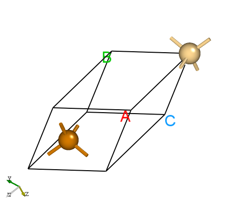
Fig.1 The primitive cell of CdTe.

Next, use VASP to optimize its lattice parameters or modify the lattice to match the experimental measurements. Users need to do it manually.

Write the required parameters in dasp.in :

############## Job Scheduling ##############
cluster = SLURM     # (job scheduling system)
node_number = 2         # (number of node)
core_per_node = 52      # (core per node)
queue = batch           # (name of queue/partition)
max_time = 24:00:00        # (maximum time for a single DFT calculation)
vasp_path_dec = /opt/vasp.5.4.4/bin/vasp_gam   #  (path of VASP)
vasp_path_tsc = /opt/vasp.5.4.4/bin/vasp_std
job_name = submit_job    # (name of script)
potcar_path = /opt/POT/potpaw_PBE    # (path of pseudopotentials)
max_job = 5

############## TSC Module ##############
database_api = ******************* # (str-list type)

############## DEC Module ##############
level = 2   # (level=1: PBE+PBE; level=2: PBE+HSE; level=3: HSE+HSE)
min_atom = 190
max_atom = 240
intrinsic = T   # (default: T)
correction = FNV   # (default: none)
epsilon = 10.3
Eg_real = 1.45   # (experimental band gap)

############## DDC Module ##############
ddc_temperature = 1000 300
ddc_mass = 0.09 0.84

Next, all the parameters listed in dasp.in will be described:

cluster = SLURM
# The system of the used cluster is SLURM.

node_number = 2
# 2 nodes are used for each calculation.

core_per_node = 52
# 52 cores are used for each node, so 2*52=104 cores are used in total for each calculation.

queue = batch
# The queue named “batch” is used to carry out calculations. Therefore, users need to make sure the queue name, nodes, and cores of clusters before configuring dasp.in.

max_time = 24:00:00        # (maximum time for a single DFT calculation)
# The maximum time allowed is 24 hours for a single DFT calculation and can be set arbitrarily.

vasp_path_dec = /opt/vasp.5.4.4/bin/vasp_gam   #  (path of VASP)
vasp_path_tsc = /opt/vasp.5.4.4/bin/vasp_std
# The VASP_std version is used for TSC calculations, and the VASP_gam version is used for DEC calculations.

job_name = submit_job    # (name of script)
# The submission script, named “submit_job” and can be set arbitrarily.

potcar_path = /opt/POT/potpaw_PBE    # (path of pseudopotentials)
# path of pseudopotentials

max_job = 5
# the allowed maximum number of jobs at the same time

database_api = ******************* # (str-list type)
# using to visit the Materials Project database

level = 2   # (level=1: PBE+PBE; level=2: PBE+HSE; level=3: HSE+HSE)
# using GGA-PBE for structural relaxation and HSE to calculate the total energy

min_atom = 190
max_atom = 240
# The number of atoms within the generated supercell that we want is between 190 and 240, and as far as possible to make a=b=c and a⊥b⊥c.

intrinsic = T   # (default: T)
# Generate intrinsic defects, V_Cd, V_Te, Cd_Te, Te_Cd, Cd_i, and Te_i.

correction = FNV   # (default: none)
# The corrections for charged defect adopt FNV correction.

epsilon = 10.3
# The dielectric constant of CdTe is 10.3.

Eg_real = 1.45   # (experimental band gap)
# The experimental band gap of CdTe is about 1.45 eV, DASP will adjust AEXX in INCAR to make the band gap of the supercell without defect equal to 1.45 eV.

ddc_temperature = 1000 300
# the growth temperature set to 1000 K and the working temperature set to 300 K.

ddc_mass = 0.09 0.84
# electron effective mass set to 0.09 and hole effective mass set to 0.84.

5.1.1.2 Use DASP to generate the required input files¶

Create a new directory CdTe, then prepare the files, POSCAR and dasp.in , mentioned above in the directory ./CdTe/. Next, execute dasp 1 to start PREPARE module and no additional operation is needed thereafter. DASP will output file 1prepare.out to record the running log of the module.

5.1.1.3 Workflow of PREPARE module¶

Generate supercell:

Firstly, the program will automatically find the optimal supercell ( as far as possible to make a=b=c and a⊥b⊥c ) based on the parameters min_atom=190 and max_atom=240 and output POSCAR for the supercell. The following are the structure messages of supercell POSCAR_nearlycube expanded by CdTe primitive cell.

Cubic_cell
1.0
19.8871435472 0.0000000000 0.0000000000
0.0000000000 19.8871435472 0.0000000000
0.0000000000 0.0000000000 19.8871435472
Cd Te
108 108
Direct
0.0000000000 0.0000000000 0.0000000000
0.8333333333 1.0000000000 0.1666666666
0.8333333333 0.1666666666 1.0000000000
0.6666666666 0.1666666666 0.1666666666
...

Through the visualization software, we can see that the included angle of the axis of the given CdTe cell is small, but the supercell generated by DASP is vertical on three sides.

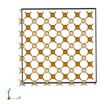
The supercell of CdTe.

Madelung constant calculation:

Secondly, according to the generated supercell, the program will execute Madelung constant calculation which describes the Coulomb interaction between charged defect and periodic image charge. (use for Lany-Zunger correction)

After finishing the above two steps calculation, the output of 1prepare.out is as follows:

############ Prepare Files module start ############

Read the structure file POSCAR you provided
Get the refined cell POSCAR_refined from POSCAR
Generate the nearlycube cell POSCAR_nearlycube from POSCAR
Generate job script through dasp.in parameters
Generate single-point KPOINTS
Generate pseudopotential file POTCAR through potcar_dir you set
Generate commonly used vasp input file INCAR
Start the madelung constant calculation
Generate the madelung calculation directory
Generate madelung calculation POSCAR
Generate madelung calculation POTCAR
Generate madelung calculation INCAR
Generate madelung calculation KPOINTS
Generate madelung calculation job script
Job 103.host5 submitted: /home/test/CdTe/dec/madelung/static
Succeed job 103.host5: /home/test/CdTe/dec/madelung/static
The madelung constant calculation completed
The madelung constant = 2.837

HSE exchange proportion calculation:

According to the generated supercell, the program will perform HSE static calculations with AEXX=0.25 and AEXX=0.3 respectively to determine the value of AEXX which can make the obtained band gap match Eg_real = 1.45 based on the slope. Therefore, after those calculations are completed, the contents in the directory CdTe/dec/AEXX/ are as follows:

cd ./dec/AEXX
ls
0.25  0.25880073638027207  0.3  AEXX.list

It indicates that the band gap of the CdTe supercell is 1.45 eV when AEXX=0.26 (two decimal places), and write this parameter into INCAR. Meanwhile, the log can be seen from 1prepare.out as follows:

Start the HSE parameter AEXX calculation
Job 107.host5 submitted: /home/test/CdTe/dec/AEXX/0.25/static
Job 108.host5 submitted: /home/test/CdTe/dec/AEXX/0.3/static
Succeed job 107.host5: /home/test/CdTe/dec/AEXX/0.25/static
Succeed job 108.host5: /home/test/CdTe/dec/AEXX/0.3/static
Job 108.host5 submitted: /home/test/CdTe/dec/AEXX/0.25880073638027207/static
Succeed job 108.host5: /home/test/CdTe/dec/AEXX/0.25880073638027207/static
The HSE parameter AEXX calculation completed
The HSE parameter AEXX = 0.26
level = 2: Generate PBE relax vasp input file INCAR-relax
level = 2: Generate HSE static vasp input file INCAR-static

Optimize the ionic position of the host supercell:

The last step in PREPARE module is to optimize the ionic position of the host supercell according to level=2 (PBE relax). The optimized file is POSCAR_final in the directory CdTe/dec/relax. At the same time, the sign of the end of DASP operation can be seen in 1prepare.out , and it also tells us that we need to do the TSC module calculation in the next step.

Start the POSCAR_nearlycube relax calculation
Generate the POSCAR_nearlycube relax directory
Job 109.host5 submitted: /home/test/CdTe/dec/relax
Succeed job 109.host5: /home/test/CdTe/dec/relax
The POSCAR_nearlycube relax calculation completed
Get the final structure POSCAR_final

############ Prepare Files module end ############

PREPARE module finished, please run DASP-TSC next

5.1.2 TSC – thermodynamic stability and chemical potential calculations¶

5.1.2.1 Run TSC module¶

The directory CdTe/dec will be created when using the command dasp 1 to execute PREPARE module, and generate file 1prepare.out in this directory. After finishing the program, there has the corresponding completion flag in 1prepare.out . Then, enter the directory CdTe/dec and confirm that the parameters in INCAR-relax and INCAR-static are feasible. (Users can modify INCAR, and DASP will make subsequent calculations based on the INCAR in this directory.)

Once confirm that the PREPARE module is finished, return to the directory CdTe and use the command dasp 2 to execute the TSC module. Similarly, the TSC module will create a directory named tsc under the directory CdTe, which contains the output of the TSC program, including every calculation directory and the running log file 2tsc.out . No additional operation is required while waiting for the program to complete.

5.1.2.2 Workflow of TSC module¶

The total energy calculation of the host structure (the parameters are consistent with MP database):

TSC module will use the same input parameters (INCAR, KPOINTS, POTCAR) with the Materials Project database to perform structural relaxation and static calculation on the primitive cells given by the user. Therefore, the calculated total energy is comparable to that of the MP database. This step is to obtain the key hetero-phases that limit the stability of CdTe. In the directory, we can see:

cd tsc
cd CdTe/
ls
relaxation1  relaxation2  static

The running log also can be seen from the CdTe/tsc/2tsc.out, that is, the steps such as generating input files, relaxation1, relaxation2, static and data extraction.

The judgement of key hetero-phases compounds:

The TSC module will search for all the secondary compounds that compete with CdTe in the MP database. And compare the total energy of CdTe calculated in the previous step with that of the hetero-phases extracted from the database to confirm CdTe is thermodynamically stable.

Subsequently, the program will automatically download the key hetero-phases compounds that can limit the thermodynamic stability of CdTe. Only Cd and Te are considered in this case. The relevant information can be seen in 2tsc.out:

...
analysing the thermodynamic stability of CdTe.
key phases of CdTe are: Cd Te .
file key_phases_info_recalc.yaml generated.
analysing of CdTe is done.
...

The total energy calculation of the host and hetero-phase compounds:

After the key hetero-phase compounds are confirmed, TSC will calculate the total energy of CdTe, Cd, and Te by using the parameter (AEXX) obtained from PREPARE module. 2tsc.out is as follows:

...
Job 112.host5 submitted: /home/test/CdTe/tsc/CdTe/static_recalc
Job 113.host5 submitted: /home/test/CdTe/tsc/Cd/static_recalc
Job 114.host5 submitted: /home/test/CdTe/tsc/Te/static_recalc
Succeed job  112.host5: /home/test/CdTe/tsc/CdTe/static_recalc
Succeed job  113.host5: /home/test/CdTe/tsc/Cd/static_recalc
Succeed job  114.host5: /home/test/CdTe/tsc/Te/static_recalc
...

The chemical potential calculation:

Calculating the formation energy and stable chemical potential region of CdTe based on the calculated total energy. As CdTe is a binary compound, TSC module will give the endpoint of two chemical potentials, i.e. Cd-rich and Te-rich, and write them into dasp.in :

# The orders are consistent with the order of elements in POSCAR, i.e. the first column is Cd and the second column is Te.
E_pure = -1.7736 -4.6974
p1 = 0.0 -1.1854
p2 = -1.1854 0.0

The output after the program is completed can be seen in 2tsc.out :

dir '2d-figures','3d-figures','ori_data_MP' ready.  try to read file: 'calc_list.yaml'.
analysing the thermodynamic stability of CdTe.
key phases of CdTe are: Cd Te .
analysing of CdTe is done.

DASP-TSC finished

For the ternary and multinary compounds, TSC module will output the image of the stable region and the chemical potential at the endpoint of the stable region.

5.1.3 DEC – the calculations of defect formation energy and transition energy level¶

5.1.3.1 Run DEC module¶

The directory CdTe/tsc will be created when using the command dasp 2 to execute TSC module, and generate file 2tsc.out in this directory. After finishing the TSC module, there has the corresponding completion flag in 2tsc.out . Then, open the file dasp.in under the directory CdTe/dasp.in to confirm the chemical potential already has been written.

Once confirm that the TSC module is finished, return to the directory CdTe and use the command dasp 3 to execute the DEC module. DEC will output relevant files in the generated directory dec in the first step, including the defect structures, directories, and the log file 3dec.out . No additional operation is required while waiting for the program to complete.

5.1.3.2 Workflow of DEC module¶

Generate defect structure:

Based on the parameter intrinsic = T in dasp.in , DEC will generate the intrinsic defects for CdTe, i.e. create the calculation directory CdTe/dec/Intrinsic_Defect, in which the structures and directories of vacancies V_Cd and V_Te, antisite defects Cd_Te and Te_Cd, as well as interstitial defects Cd_i and Te_i are included. According to the crystal symmetry analysis, there has no inequivalent site for Cd and Te in CdTe lattice, thus only one configuration needs to be generated for each kind of defect.

cd dec/Intrinsic_Defect/
ls
Cd_i  Cd_Te1  host  Intrinsic_Defect.list  Te_Cd1  Te_i  V_Cd1  V_Te1

At the same time, the output of DEC module can be seen in 3dec.out as follows:

############ Neutral Defect module start ############
Make intrinsic defect directory Intrinsic_Defect
Generate host directory in Intrinsic_Defect
Start generating neutral vacancy defect
Generate neutral defect at: V_Cd1/initial_structure/q0
Generate neutral defect at: V_Te1/initial_structure/q0
Neutral vacancy defect generation completed
Start generating neutral intrinsic antisite defect
Generate neutral defect at: Te_Cd1/initial_structure/q0
Generate neutral defect at: Cd_Te1/initial_structure/q0
Neutral intrinsic antisite defect generation completed
Start generating neutral intrinsic interstitial defect
Generate neutral defect at: Cd_i/random1/initial_structure/q0
Generate neutral defect at: Cd_i/random2/initial_structure/q0
Generate neutral defect at: Cd_i/random3/initial_structure/q0
Generate neutral defect at: Cd_i/random4/initial_structure/q0
Generate neutral defect at: Cd_i/random5/initial_structure/q0
Generate neutral defect at: Cd_i/random6/initial_structure/q0
Generate neutral defect at: Te_i/random1/initial_structure/q0
Generate neutral defect at: Te_i/random2/initial_structure/q0
Generate neutral defect at: Te_i/random3/initial_structure/q0
Generate neutral defect at: Te_i/random4/initial_structure/q0
Generate neutral defect at: Te_i/random5/initial_structure/q0
Generate neutral defect at: Te_i/random6/initial_structure/q0
Neutral intrinsic interstitial defect generation completed

############ Neutral Defect module end ############

It can be seen that the DEC module only creates the directories for all the neutral defects at this time.

Submit jobs for all defects with q=0:

After the structures and directories of neutral defects are generated, DEC module will call VASP to perform structural relaxation with PBE and total energy calculation with HSE (corresponds to the parameter level = 2 in dasp.in ), this step may need a long time. Users can check the file 3dec.out at any time. The messages in 3dec.out are as follows:

Job 245.host5 submitted: /home/test/CdTe/dec/Intrinsic_Defect/Cd_Te1/initial_structure/q0
Job 246.host5 submitted: /home/test/CdTe/dec/Intrinsic_Defect/Te_Cd1/initial_structure/q0
Job 247.host5 submitted: /home/test/CdTe/dec/Intrinsic_Defect/V_Te1/initial_structure/q0
Job 248.host5 submitted: /home/test/CdTe/dec/Intrinsic_Defect/Te_i/random3/initial_structure/q0
Job 249.host5 submitted: /home/test/CdTe/dec/Intrinsic_Defect/Te_i/random2/initial_structure/q0
Failed job 245.host5: /home/test/CdTe/dec/Intrinsic_Defect/Cd_Te1/initial_structure/q0
...

It can be seen that there occur some mistakes in the structural relaxation for the neutral Cd_Te1 which leads to the calculation can not complete. But the program is not interrupted and will continue to finish the calculations except for Cd_Te. Therefore, users need to do nothing and wait for the program to complete. (the problems about defect Cd_Te will be solved after the program is completed.) If encountered the VASP error, please see Common Problems and Solutions.

Generate calculation directories for the charged defects:

After finishing the calculations of all the neutral defects (except for Cd_Te and interstitial with high energy), the program will judge the charge states of each defect and generate the corresponding directories and files for the charged defects based on the results of the neutral defects. A prompt will be given for those defects with calculation errors (undo, failed, and not converged) or without subsequent calculation (skip). The relevant information in 3dec.out is as follows:

############ Ionized Defect module start ############
Start generating ionized defects
Warning: no EIGENVAL in /home/test/CdTe/dec/Intrinsic_Defect/Cd_Te1/initial_structure/q0/static, skipped this directory!
Start generating ionized defects
Ionized defect path: /home/test/CdTe/dec/Intrinsic_Defect/V_Te1/initial_structure/q+1
Ionized defect path: /home/test/CdTe/dec/Intrinsic_Defect/V_Te1/initial_structure/q+2
Ionized defects generation completed
Start generating ionized defects
Ionized defect path: /home/test/CdTe/dec/Intrinsic_Defect/Te_i/random3/initial_structure/q+1
Ionized defect path: /home/test/CdTe/dec/Intrinsic_Defect/Te_i/random3/initial_structure/q+2
Ionized defect path: /home/test/CdTe/dec/Intrinsic_Defect/Te_i/random3/initial_structure/q+3
Ionized defect path: /home/test/CdTe/dec/Intrinsic_Defect/Te_i/random3/initial_structure/q+4
...

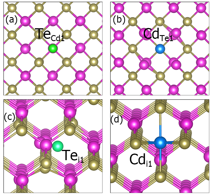
Take some defect structures to see in the visualization software, as shown in below:

Part of defect structures of CdTe.

Submit jobs for the defects with q≠0:

After the structures and directories of the charged defects are generated, DEC module will call VASP to perform structural relaxation with PBE and total energy calculation with HSE (corresponds to the parameter level = 2 in dasp.in ). The waiting time needed in this step will be longer than that in 3.2.2. The messages in 3dec.out are as follows:

############ AutoRun - Ionized Defect module start ############
Job 693.host5 submitted: /home/test/CdTe/dec/Intrinsic_Defect/V_Te1/initial_structure/q+2
Job 694.host5 submitted: /home/test/CdTe/dec/Intrinsic_Defect/V_Te1/initial_structure/q+1
Job 695.host5 submitted: /home/test/CdTe/dec/Intrinsic_Defect/Te_i/random3/initial_structure/q+2
Job 696.host5 submitted: /home/test/CdTe/dec/Intrinsic_Defect/Te_i/random3/initial_structure/q+1
Job 700.host5 submitted: /home/test/CdTe/dec/Intrinsic_Defect/Te_i/random3/initial_structure/q+4
Succeed job 694.host5: /home/test/CdTe/dec/Intrinsic_Defect/V_Te1/initial_structure/q+1
Succeed job 693.host5: /home/test/CdTe/dec/Intrinsic_Defect/V_Te1/initial_structure/q+2
...

Calculate the correction for the charged defects:

After finishing the calculations of all the charged defects (except for Cd_Te), DEC module will calculate the FNV correction (according to the parameter correction = FNV in dasp.in ), and then the formation energies and transition energy levels are also calculated. The specific data of the corrections and formation energies of different charge states of each defect are recorded in file 3dec.out :

...
The formation energy (neutral) of V_Te1 at p1 is 1.684321
The formation energy (neutral) of V_Te1 at p2 is 2.869721
The FNV correction (q = 2) E_correct =  0.279795 eV
The transition level (0/2+) above VBM: 1.2429
The FNV correction (q = 1) E_correct =  0.087991 eV
The transition level (0/+) above VBM: 1.2833
...

All the data related to formation energies and transition energy levels are also recorded in the file defect.log under each defect’s corresponding directories.

Output the image of formation energy:

Up to now, the program has already been completed, but we find the defect Cd_Te were not calculated by the output. The solution is as follows:
According to the error information, adjust the parameters in INCAR in the directory /home/test/CdTe/dec/Intrinsic_Defect/Cd_Te1/initial_structure/q0.
Return to the directory dec and create a new file named redo.in , and write /home/test/CdTe/dec/Intrinsic_Defect/Cd_Te1/initial_structure/q0.
Return to the directory CdTe and execute the DEC module again with the command dasp 3 . The program will automatically judge the completed calculations, and recalculate the defect according to the redo.in .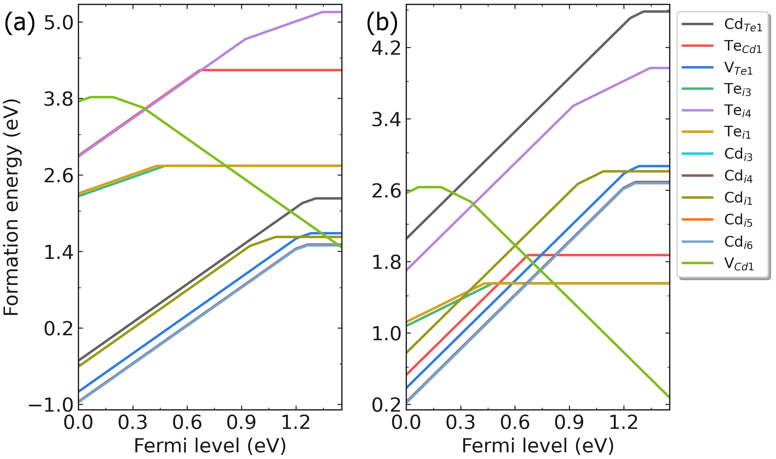
The DEC module will carry out the calculations for the neutral and charged defect of Cd_Te, and calculate their formation energies.

Finally, DEC will automatically outputs the image of defect formation energy v.s. Fermi level by using all the corrected defect formation energies of CdTe at two chemical potentials. As shown in below:

Fig: Formation energies of intrinsic defects in CdTe as functions of Fermi level under (a) Cd-rich and (b) Te-rich conditions.

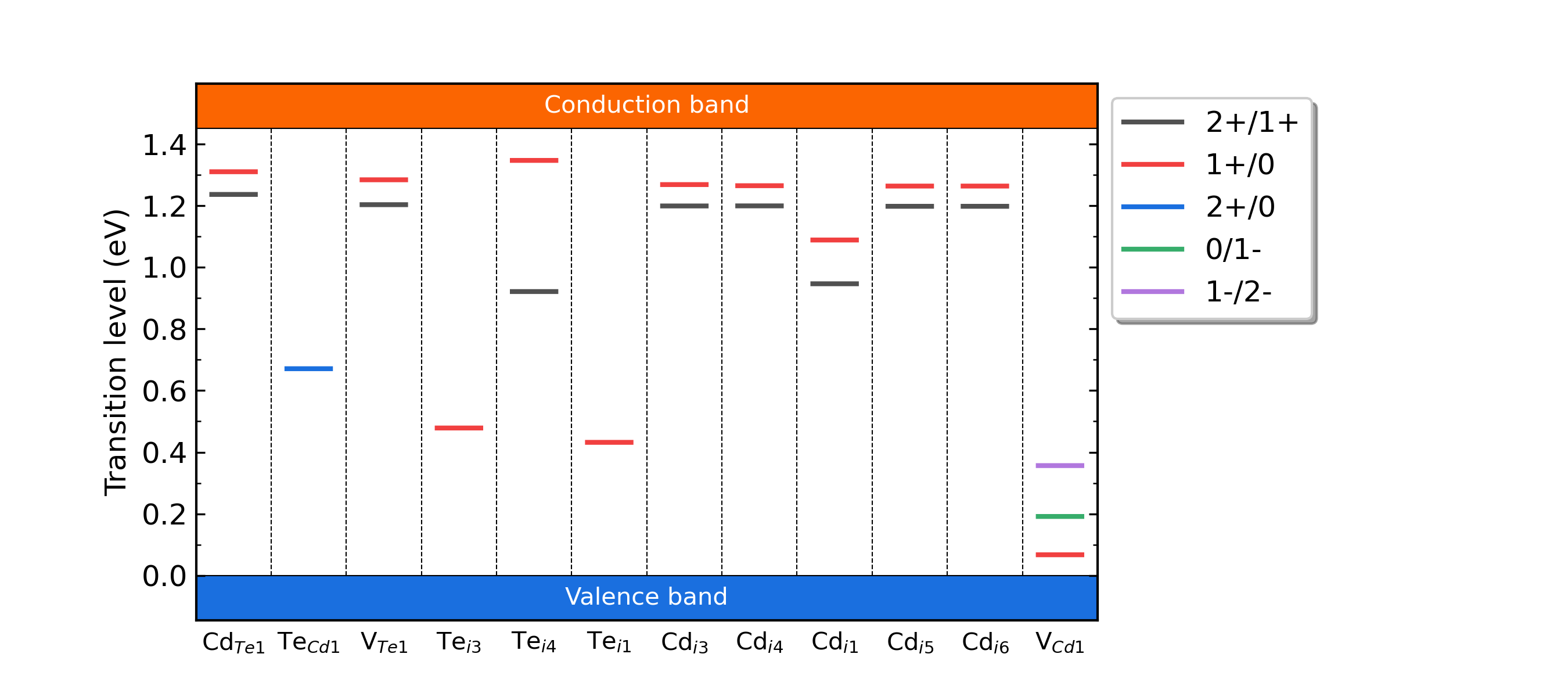
Fig: The charge-state transition energy levels of intrinsic defects in CdTe.

5.1.4 DDC – defect density and Fermi level calculations¶

5.1.4.1 Run DDC module¶

After finishing the DEC module, return to the directory CdTe and use the command dasp 4 to execute the DDC module. No additional operation is required while waiting for the program to complete.

5.1.4.2 Workflow of DDC module¶

Firstly, DDC module will judge which defects have been finished calculating based on the output of DEC module, and take all these defects into consideration in the DDC calculation. Then, DDC will search for the output information about each defect as formation energy, transition energy levels, and degeneracy factor. Finally, summarize all the data and write in the file DefectParams.txt .

4ddc.out is the log file of DDC module：

############ Collecting information from DEC ############
Read defect types from DEC calculation successfully.
Defects considered in DDC calculation: ['Cd_Te1', 'Te_Cd1', 'V_Te1', 'Te_i-3', 'Te_i-4', 'Te_i-1', 'Cd_i-3', 'Cd_i-4', 'Cd_i-1', 'Cd_i-5', 'Cd_i-6', 'V_Cd1']
Chemical potentials change from p1 to p2.
Calculate gq for defect in each charge state.
Calculate Nsites for Cd_Te1: 1.373114e+22 cm^-3.
Calculate Nsites for Te_Cd1: 1.373114e+22 cm^-3.
Calculate Nsites for V_Te1: 1.373114e+22 cm^-3.
Calculate Nsites for Te_i-3: 9.154092e+21 cm^-3.
Calculate Nsites for Te_i-4: 9.154092e+21 cm^-3.
Calculate Nsites for Te_i-1: 9.154092e+21 cm^-3.
Calculate Nsites for Cd_i-3: 9.154092e+21 cm^-3.
Calculate Nsites for Cd_i-4: 9.154092e+21 cm^-3.
Calculate Nsites for Cd_i-1: 9.154092e+21 cm^-3.
Calculate Nsites for Cd_i-5: 9.154092e+21 cm^-3.
Calculate Nsites for Cd_i-6: 9.154092e+21 cm^-3.
Calculate Nsites for V_Cd1: 1.373114e+22 cm^-3.
############ Collecting information from DEC ############

Below is the file DefectParams.txt :

1000 300
0.090000 0.840000
1.454001
Cd_Te1 1.373114e+22 1 1.3094 2 1.2726 1 x x x x x x x x x x x x 2.230998 4.601798
Te_Cd1 1.373114e+22 1 0.4662 2 0.6708 1 0.3386 2 0.1484 1 x x x x x x x x 4.243870 1.873070
V_Te1 1.373114e+22 1 1.2833 2 1.2429 1 x x x x x x x x x x x x 1.684321 2.869721
Te_i-3 9.154092e+21 1 0.4786 2 0.153 1 0.1435 2 0.012 1 x x x x x x x x 2.743050 1.557650
Te_i-4 9.154092e+21 1 1.3461 2 1.1335 1 0.6062 2 0.4609 1 x x x x x x x x 5.154681 3.969281
Te_i-1 9.154092e+21 1 0.432 2 0.1299 1 0.0022 2 -0.0831 1 x x x x x x x x 2.740914 1.555514
Cd_i-3 9.154092e+21 1 1.2677 2 1.2331 1 0.7237 2 0.4498 1 x x x x x x x x 1.506642 2.692042
Cd_i-4 9.154092e+21 1 1.2641 2 1.2314 1 0.7192 2 0.4466 1 x x x x x x x x 1.505396 2.690796
Cd_i-1 9.154092e+21 1 1.0881 2 1.0171 1 0.5865 2 0.3569 1 x x x x x x x x 1.626088 2.811488
Cd_i-5 9.154092e+21 1 1.2629 2 1.2301 1 0.7187 2 0.4461 1 x x x x x x x x 1.493426 2.678826
Cd_i-6 9.154092e+21 1 1.2629 2 1.2301 1 0.7187 2 0.4461 1 x x x x x x x x 1.493426 2.678826
V_Cd1 1.373114e+22 1 0.0676 2 0.0115 1 -0.0427 2 -0.0964 1 0.1918 2 0.2742 1 0.7753 2 1.0413 1 3.819933 2.634533

Self-consistent calculation under growth temperature:

The DDC module will calculate the defect/dopant and carrier densities at the temperature T=1000 K ( ddc_temperature = 1000 300 ), and obtain the Fermi level by self-consistently under the charge neutralization condition.

Self-consistent calculation under working (measuring) temperature:

The DDC module will recalculate the defect/dopant and carrier densities at the temperature T=300 K ( ddc_temperature = 1000 300 ), and re-obtain the Fermi level by self-consistently under the charge neutralization condition.

Output defect density:

DDC module will output four files in the directory CdTe/ddc: Fermi.dat , Carrier.dat , Defect_charge.dat , and density.png . Using different growth temperatures, the images density.png are as follows:

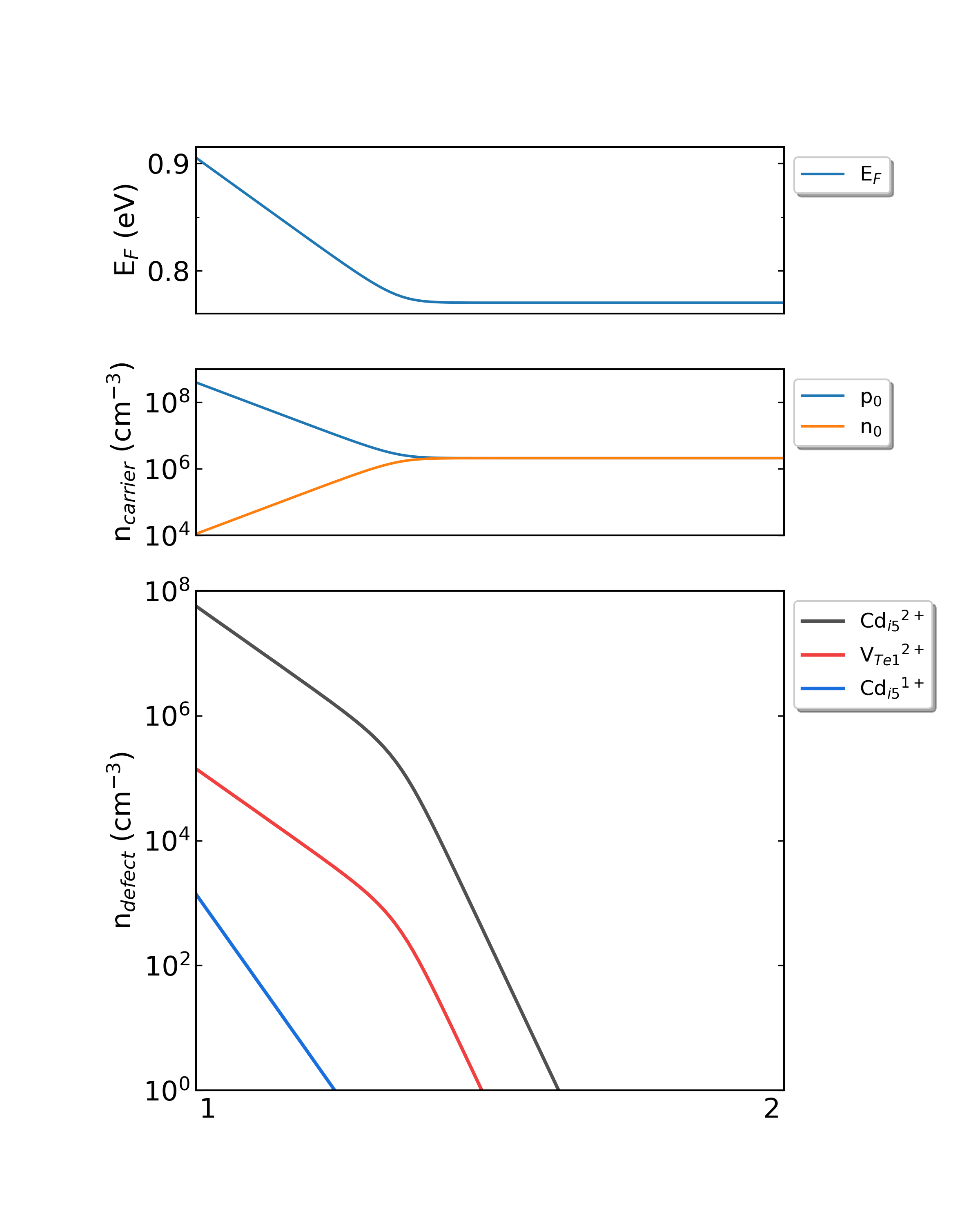
Fig: The Fermi level, electron and hole carrier densities, and defect densities in CdTe as functions of the chemical potentials with the growth temperature is 300 K and the working temperature is 300 K.

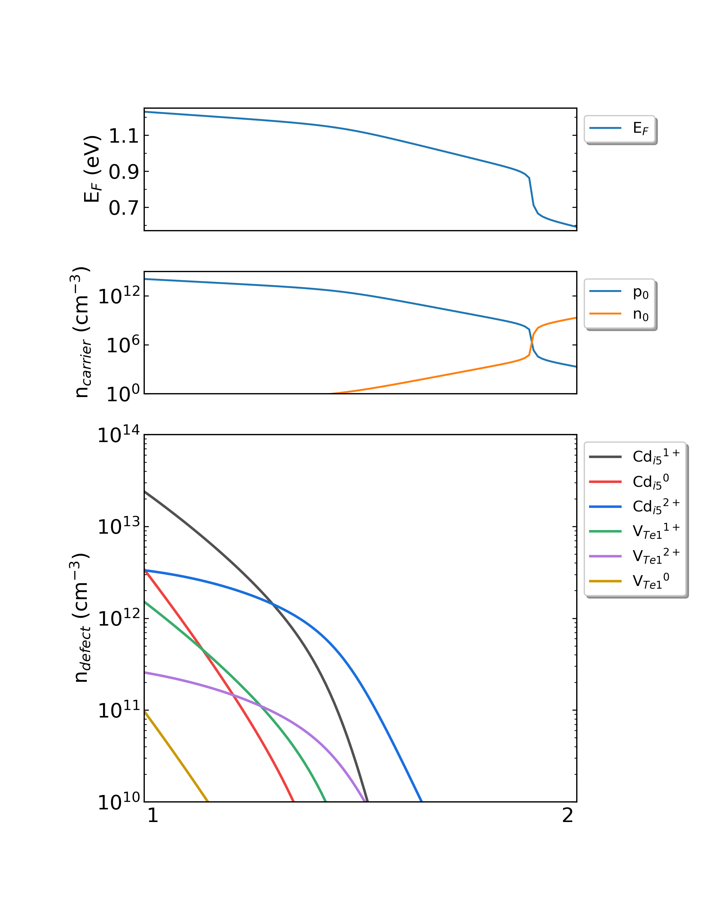
Fig: The Fermi level, electron and hole carrier densities, and defect densities in CdTe as functions of the chemical potentials with the growth temperature is 600 K and the working temperature is 300 K.

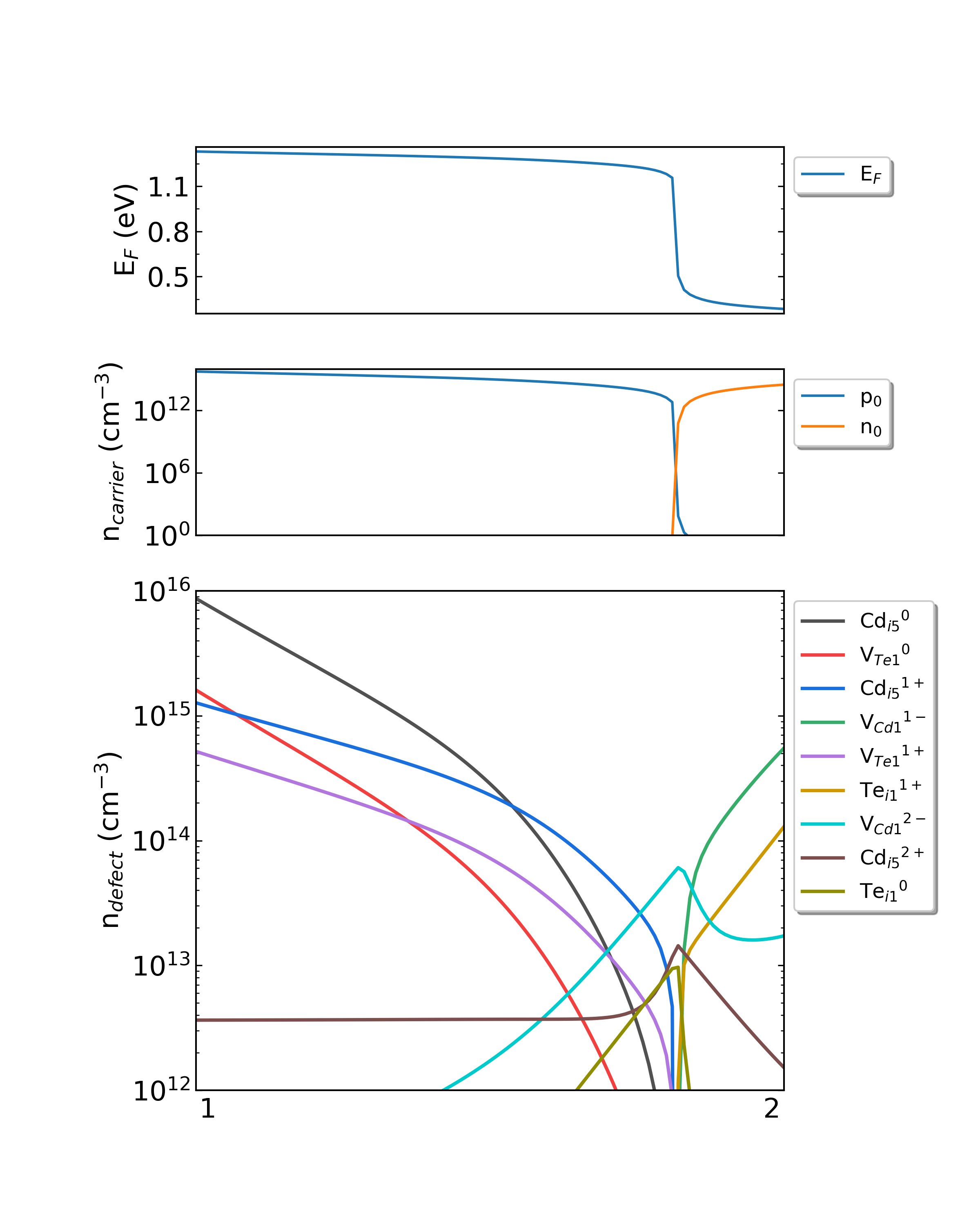
Fig: The Fermi level, electron and hole carrier densities, and defect densities in CdTe as functions of the chemical potentials with the growth temperature is 1000 K and the working temperature is 300 K.

5.2 The calculations of intrinsic defects in HfO2¶

HfO2 is an important material widely used in electronic devices with a high dielectric constant. Recently, it has attracted a lot of attention as its metastable phase possesses ferroelectric. The defects in HfO2 may affect its phase stability, and dielectric and ferroelectric properties, so it is necessary to systematically calculate the defect properties of HfO2.
With the help of the efficient software DASP, the properties of the point defects and the relationship between the defects formation and its phase stability in HfO2 can be systematically studied.
The following is an example of using DASP to calculate intrinsic defects in HfO2:

5.2.1 PREPARE — Prepares for calculation¶

5.2.1.1 POSCAR and dasp.in¶

Find the POSCAR for HfO2 from the Materials Project database, as follows:

 Hf4 O8
00000000000000
          5.0652456351012756    0.0000000000000000   -0.8648023964655065
          0.0000000000000000    5.1942160710694010    0.0000000000000000
         -0.0006123763055649    0.0000000000000000    5.3264852554835196
Hf   O
  8
Direct
7239198560286844  0.5430528338948646  0.2919471319794364
2760801439713155  0.0430528338948647  0.2080528680205637
2760801439713155  0.4569471661051352  0.7080528680205705
7239198560286844  0.9569471661051354  0.7919471319794295
5514108623083260  0.2575137054162841  0.0226462276199697
4485891376916739  0.7575137054162840  0.4773537723800304
4485891376916739  0.7424862945837160  0.9773537723800304
5514108623083260  0.2424862945837159  0.5226462276199696
9317881306845183  0.6693565882783469  0.6530354073676818
0682118693154819  0.1693565882783468  0.8469645926323182
0682118693154819  0.3306434117216532  0.3469645926323183
9317881306845183  0.8306434117216531  0.1530354073676817

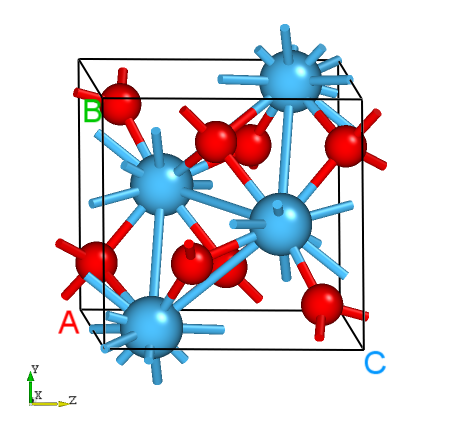
Taking it into the crystal visualization software, the structure can be seen as below:

The structure of HfO2.

Next, use VASP to optimize its lattice parameters or modify the lattice to match the experimental measurements. Users need to do it manually.

Write the required parameters in dasp.in :

############## Job Scheduling ##############
cluster = PBS     # (job scheduling system)
node_number = 1         # (number of node)
core_per_node = 96      # (core per node)
queue = batch           # (name of queue/partition)
max_time = 24:00:00        # (maximum time for a single DFT calculation)
vasp_path_dec = /opt/vasp.5.4.4/bin/vasp_gam   #  (path of VASP)
vasp_path_tsc = /opt/vasp.5.4.4/bin/vasp_std
job_name = submit_job    # (name of script)
potcar_path = /opt/POT/potpaw_PBE    # (path of pseudopotentials)
max_job = 5

############## TSC Module ##############
database_api = ******************* # (str-list type)

############## DEC Module ##############
level = 2   # (level=1: PBE+PBE; level=2: PBE+HSE; level=3: HSE+HSE)
min_atom = 96
max_atom = 96
intrinsic = T   # (default: T)
correction = FNV   # (default: none)
epsilon = 10.3
Eg_real = 1.45   # (experimental band gap)

############## DDC Module ##############
ddc_temperature = 800 300
ddc_mass = 2.95 2.99

Next, all the parameters listed in dasp.in will be described:

cluster = PBS
# The system of the used cluster is PBS.

node_number = 1
# One node is used for each calculation.

core_per_node = 96
# 96 cores are used for each node, so 1*96=96 cores are used in total for each calculation.

queue = batch
# The queue named “batch” is used to carry out calculations. Therefore, users need to make sure the queue name, nodes, and cores of clusters before configuring dasp.in.

max_time = 24:00:00        # (maximum time for a single DFT calculation)
# The maximum time allowed is 24 hours for a single DFT calculation and can be set arbitrarily.

vasp_path_dec = /opt/vasp.5.4.4/bin/vasp_gam   #  (path of VASP)
vasp_path_tsc = /opt/vasp.5.4.4/bin/vasp_std
# The VASP_std version is used for TSC calculations, and the VASP_gam version is used for DEC calculations.

job_name = submit_job    # (name of script)
# The submission script, named “ submit_job” and can be set arbitrarily.

potcar_path = /opt/POT/potpaw_PBE    # (path of pseudopotentials)
# path of pseudopotentials

max_job = 5
# the allowed maximum number of jobs at the same time

database_api = ******************* # (str-list type)
# using to visit the Materials Project database

level = 2   # (level=1: PBE+PBE; level=2: PBE+HSE; level=3: HSE+HSE)
# using GGA-PBE for structural relaxation and HSE to calculate the total energy

min_atom = 96
max_atom = 96
# The number of atoms within the generated supercell that we want is 96, and as far as possible to make a=b=c and a⊥b⊥c.

intrinsic = T   # (default: T)
# Generate intrinsic defects, V_Hf, V_O, Hf_O, O_Hf, Hf_i, and O_i.

correction = FNV   # (default: None)
# Generate intrinsic defects, V_Hf, V_O, Hf_O, O_Hf, Hf_i, and O_i.

epsilon = 21.6
# The dielectric constant of HfO2 is 21.6.

Eg_real = 5.68   # (experimental band gap)
# The experimental band gap of HfO2 is about 5.68 eV, DASP will adjust AEXX in INCAR to make the band gap of the supercell without defect equal to 5.68 eV.

ddc_temperature = 1000 300
# the growth temperature set to 1000 K and the working temperature set to 300 K.

ddc_mass = 2.95 2.99
# electron effective mass set to 2.95 and hole effective mass set to 2.99.

5.2.1.2 Use DASP to generate the required input files¶

Create a new directory HfO2, then prepare the files, POSCAR and dasp.in , mentioned above in the directory ./HfO2/. Next, execute dasp 1 to start PREPARE module and no additional operation is needed thereafter. DASP will output file 1prepare.out to record the running log of the module.

5.2.1.3 Workflow of PREPARE module¶

Generate supercell:

Firstly, the program will automatically find the optimal supercell ( as far as possible to make a=b=c and a⊥b⊥c ) based on the parameters min_atom=96 and max_atom=96 and output POSCAR for the supercell. The following are the structure messages of HfO2 supercell POSCAR_nearlycube .

Cubic_cell
1.0
10.2770806222 0.0000000000 0.0000000000
0.0000000000 10.3884321420 0.0000000000
-1.7940733247 0.0000000000 10.5008134501
Hf O
32 64
Direct
0.3619599280 0.2715264169 0.1459735659
0.1380400719 0.0215264169 0.1040264340
0.1380400719 0.2284735830 0.3540264340
0.3619599280 0.4784735830 0.3959735659

...

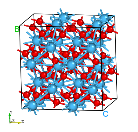
Taking it into the crystal visualization software, the supercell can be seen as below:

Fig: The structure of HfO2 supercell generated by DASP.

Madelung constant calculation:

Secondly, according to the generated supercell file, the program will execute Madelung constant calculation which describes the Coulomb interaction between charged defect and periodic image charge.

After finishing the above two steps calculation, the output of 1prepare.out is as follows:

############ Prepare Files module start ############

Read the structure file POSCAR you provided
Get the refined cell POSCAR_refined from POSCAR
Generate the nearlycube cell POSCAR_nearlycube from POSCAR
Generate job script through dasp.in parameters
Generate single-point KPOINTS
Generate pseudopotential file POTCAR through potcar_dir you set
Generate commonly used vasp input file INCAR
Start the madelung constant calculation
Generate the madelung calculation directory
Generate madelung calculation POSCAR
Generate madelung calculation POTCAR
Generate madelung calculation INCAR
Generate madelung calculation KPOINTS
Generate madelung calculation job script
Job 103.host5 submitted: /home/fudan/HfO2/dec/madelung/static
Succeed job 103.host5: /home/fudan/HfO2/dec/madelung/static
The madelung constant calculation completed
The madelung constant = 2.841

HSE exchange proportion calculation:

According to the generated supercell file, the program will perform HSE static calculations with AEXX=0.25 and AEXX=0.3 respectively to determine the value of AEXX which can make the obtained band gap match Eg_real = 5.68 based on the slope. If the calculated band gap with AEXX=0.25 or AEXX=0.3 is consistent with the set, the subsequent calculation for AEXX will not be performed. This is the example where the bandgap is satisfied when AEXX=0.25. Therefore, after the calculation is completed, the contents in the directory HfO2/dec/AEXX/ are as follows:

cd ./dec/AEXX
ls
0.25  AEXX.list

It indicates that the band gap of the HfO2 supercell is 5.68 eV when AEXX=0.25 (two decimal places), and write this parameter into INCAR. Meanwhile, the log can be seen from 1prepare.out as follows:

Start the HSE parameter AEXX calculation
Job 107.host5 submitted: /home/fudan/HfO2/dec/AEXX/0.25/static
Succeed job 107.host5: /home/fudan/HfO2/dec/AEXX/0.25/static
The HSE parameter AEXX calculation completed
The HSE parameter AEXX = 0.25
level = 2: Generate PBE relax vasp input file INCAR-relax
level = 2: Generate HSE static vasp input file INCAR-static

Optimize the ionic position of the host supercell:

The last step in PREPARE module is to optimize the ionic position of the host supercell according to level=2 (i.e. PBE relax). The optimized file is POSCAR_final in the directory HfO2/dec/relax. At the same time, the sign of the end of DASP operation can be seen in 1prepare.out , and it also tells us that we need to do the TSC module calculation in the next step.

Start the POSCAR_nearlycube relax calculation
Generate the POSCAR_nearlycube relax directory
Job 110.host5 submitted: /home/fudan/HfO2/dec/relax
Succeed job 110.host5: /home/fudan/HfO2/dec/relax
The POSCAR_nearlycube relax calculation completed
Get the final structure POSCAR_final

############ Prepare Files module end ############

DASP-PREPARE finished, please run DASP-TSC next

5.2.2 TSC – thermodynamic stability and chemical potential calculations¶

5.2.2.1 Run TSC module¶

The directory HfO2/dec will be created when using the command dasp 1 to execute PREPARE module, and generate file 1prepare.out in this directory. After finishing the program, there has the corresponding completion flag in 1prepare.out . Then, enter the directory HfO2/dec and confirm that the parameters in INCAR-relax and INCAR-static are feasible. (Users can modify INCAR, and DASP will make subsequent calculations based on the INCAR in this directory.)

Once confirm that the PREPARE module is finished, return to the directory HfO2 and use the command dasp 2 to execute the TSC module. Similarly, the TSC module will create a directory named tsc under the directory HfO2, which contains the output of the TSC program, including every calculation directory and the running log file 2tsc.out . No additional operation is required while waiting for the program to complete.

5.2.2.2 Workflow of TSC module¶

The total energy calculation of the host structure (the parameters are consistent with MP database):

TSC module will use the same input parameters (INCAR, KPOINTS, POTCAR) with the Materials Project database to perform structural relaxation and static calculation on the primitive cells given by the user. Therefore, the calculated total energy is comparable to that of the MP database. This step is to obtain the key hetero-phases that limit the stability of HfO2. In the directory, we can see:

cd tsc
cd HfO2/
ls
relaxation1  relaxation2  static

The running log also can be seen from the HfO2/tsc/2tsc.out, that is, the steps such as generating input files, relaxation1, relaxation2, static and data extraction.

The judgement of key hetero-phases compounds:

The TSC module will search for all the secondary compounds that compete with HfO2 in the MP database. And compare the total energy of HfO2 calculated in the previous step with that of the hetero-phases extracted from the database to confirm HfO2 is thermodynamically stable.

Subsequently, the program will automatically download the key hetero-phase compounds that can limit the thermodynamic stability of HfO2. Only Hf and O2 are considered in this case. The relevant information can be seen in 2tsc.out :

...
analysing the thermodynamic stability of HfO2.
key phases of HfO2 are: Hf O2 .
file key_phases_info_recalc.yaml generated.
analysing of HfO2 is done.
...

The total energy calculation of the host and hetero-phase compounds:

After the key hetero-phase compounds are confirmed, TSC will calculate the total energy of HfO2, Hf, and O2 by using the parameter (AEXX) obtained from PREPARE module. 2tsc.out is as follows:

...
Job 182.host5 submitted: /home/test/HfO2/tsc/HfO2/static_recalc
Job 183.host5 submitted: /home/test/HfO2/tsc/Hf/static_recalc
Job 184.host5 submitted: /home/test/HfO2/tsc/O2/static_recalc
Succeed job  182.host5: /home/test/HfO2/tsc/HfO2/static_recalc
Succeed job  183.host5: /home/test/HfO2/tsc/Hf/static_recalc
Succeed job  184.host5: /home/test/HfO2/tsc/O2/static_recalc
...

The chemical potential calculation:

Calculating the formation energy and stable chemical potential region of HfO2 based on the calculated total energy. As HfO2 is a binary compound, TSC module will give the endpoint of two chemical potentials, i.e. Hf-rich and O-rich, and write them into dasp.in :

# The orders are consistent with the order of elements in POSCAR, i.e. the first column is Hf and the second column is O.
E_pure = -11.1092 -8.2689
p1 = 0.0 -5.8748
p2 = -11.7496 0.0

The output after the program is completed can be seen in 2tsc.out :

dir '2d-figures','3d-figures','ori_data_MP' ready.  try to read file: 'calc_list.yaml'.
analysing the thermodynamic stability of HfO2.
key phases of HfO2 are: Hf O2 .
analysing of HfO2 is done.
---------------------------
DASP-TSC finished

For the ternary and multinary compounds, TSC module will output the image of the stable region and the chemical potential at the endpoint of the stable region.

5.2.3 DEC – the calculations of defect formation energy and transition energy level¶

5.2.3.1 Run DEC module¶

The directory HfO2/tsc will be created when using the command dasp 2 to execute TSC module, and generate file 2tsc.out in this directory. After finishing the TSC module, there has the corresponding completion flag in 2tsc.out . Then, open the file dasp.in under the directory HfO2/dasp.in to confirm the chemical potential already has been written.

Once confirm that the TSC module is finished, return to the directory HfO2 and use the command dasp 3 to execute the DEC module. DEC will output relevant files in the generated directory dec in the first step, including the defect structures, directories, and the log file 3dec.out . No additional operation is required while waiting for the program to complete.

5.2.3.2 Workflow of DEC module¶

Generate defect structure:

Based on the parameter intrinsic = T in dasp.in , DEC will generate the intrinsic defects for HfO2, i.e. create the calculation directory HfO2e/dec/Intrinsic_Defect, in which the structures and directories of vacancies V_Hf and V_O, antisite defects Hf_O and O_Hf, as well as interstitial defects Hf_i and O_i are included. According to the crystal symmetry analysis, there has no inequivalent site for Hf atom, but two inequivalent sites for O atom. Therefore, there will generate two different configurations for V_O and Hf_O and one configuration for V_Hf and O_Hf, while the number of configurations for Hf_i and O_i is depended on the input parameter set by users.

cd dec/Intrinsic_Defect/
ls
Hf_i  Hf_O1  Hf_O2  host  Intrinsic_Defect.list  O_Hf1  O_i  V_Hf1  V_O1  V_O2

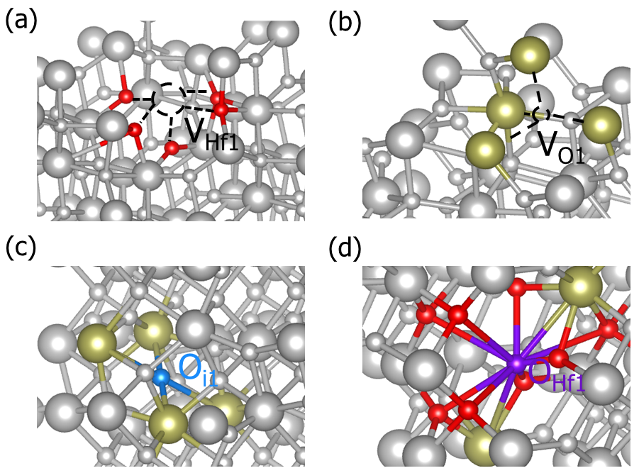
Take some defect structures to see in the visualization software, as shown in below:

Part of defect structures of HfO2.

At the same time, the output of DEC module can be seen in 3dec.out as follows:

############ Neutral Defect module start ############

Make intrinsic defect directory Intrinsic_Defect
Generate host directory in Intrinsic_Defect
Start generating neutral vacancy defect
Generate neutral defect at: V_Hf1/initial_structure/q0
Generate neutral defect at: V_O1/initial_structure/q0
Generate neutral defect at: V_O2/initial_structure/q0
Neutral vacancy defect generation completed
Start generating neutral intrinsic antisite defect
Generate neutral defect at: O_Hf1/initial_structure/q0
Generate neutral defect at: Hf_O1/initial_structure/q0
Generate neutral defect at: Hf_O2/initial_structure/q0
Neutral intrinsic antisite defect generation completed
Start generating neutral intrinsic interstitial defect
Generate neutral defect at: Hf_i/random1/initial_structure/q0
Generate neutral defect at: Hf_i/random2/initial_structure/q0
Generate neutral defect at: Hf_i/random3/initial_structure/q0
Generate neutral defect at: Hf_i/random4/initial_structure/q0
Generate neutral defect at: Hf_i/random5/initial_structure/q0
Generate neutral defect at: Hf_i/random6/initial_structure/q0
Generate neutral defect at: O_i/random1/initial_structure/q0
Generate neutral defect at: O_i/random2/initial_structure/q0
Generate neutral defect at: O_i/random3/initial_structure/q0
Generate neutral defect at: O_i/random4/initial_structure/q0
Generate neutral defect at: O_i/random5/initial_structure/q0
Generate neutral defect at: O_i/random6/initial_structure/q0
Neutral intrinsic interstitial defect generation completed

############ Neutral Defect module end ############

It can be seen that the DEC module only creates the directories for all the neutral defects at this time.

Submit jobs for all defects with q=0:

After the structures and directories of neutral defects are generated, DEC module will call VASP to perform structural relaxation with PBE and total energy calculation with HSE (corresponds to the parameter level=2 in dasp.in ), this step may need a long time. Users can check the file 3dec.out at any time. The messages in 3dec.out are as follows:

Job 198.host5 submitted: /data/HfO2/dec/Intrinsic_Defect/V_O2/initial_structure/q0
Job 200.host5 submitted: /data/HfO2/dec/Intrinsic_Defect/V_O1/initial_structure/q0
Job 202.host5 submitted: /data/HfO2/dec/Intrinsic_Defect/O_Hf1/initial_structure/q0
Job 204.host5 submitted: /data/HfO2/dec/Intrinsic_Defect/Hf_O1/initial_structure/q0
Job 206.host5 submitted: /data/HfO2/dec/Intrinsic_Defect/Hf_i/random5/initial_structure/q0

...

Succeed job 202.host5: /data/HfO2/dec/Intrinsic_Defect/O_Hf1/initial_structure/q0
Succeed job 198.host5: /data/HfO2/dec/Intrinsic_Defect/V_O2/initial_structure/q0
Failed job 204.host5: /data/HfO2/dec/Intrinsic_Defect/Hf_O1/initial_structure/q0
Succeed job 206.host5: /data/HfO2/dec/Intrinsic_Defect/Hf_i/random5/initial_structure/q0

...

It can be seen that there occur some mistakes in the structural relaxation for the neutral Hf_O1 which leads to the calculation can not complete. But the program is not interrupted and will continue to finish the calculations except for Hf_O1. Therefore, users need to do nothing and wait for the program to complete. (the problems about defect Hf_O will be solved after the program is completed.) If encountered the VASP error, please see Common Problems and Solutions.

Generate calculation directories for the charged defects:

After finishing the calculations of all the neutral defects (except for Hf_O and interstitial with high energy), the program will judge the charge states of each defect and generate the corresponding directories and files for the charged defects based on the results of the neutral defects. A prompt will be given for those defects with calculation errors (undo, failed, and not converged) or without subsequent calculation (skip). The relevant information in 3dec.out is as follows:

############ Ionized Defect module start ############
Start generating ionized defects
Ionized defect path: /data/HfO2/dec/Intrinsic_Defect/Hf_O2/initial_structure/q+1
Ionized defect path: /data/HfO2/dec/Intrinsic_Defect/Hf_O2/initial_structure/q+2
Ionized defect path: /data/HfO2/dec/Intrinsic_Defect/Hf_O2/initial_structure/q+3
Ionized defect path: /data/HfO2/dec/Intrinsic_Defect/Hf_O2/initial_structure/q+4
Ionized defects generation completed
Start generating ionized defects
Ionized defect path: /data/HfO2/dec/Intrinsic_Defect/V_O2/initial_structure/q-2
Ionized defect path: /data/HfO2/dec/Intrinsic_Defect/V_O2/initial_structure/q-1
Ionized defect path: /data/HfO2/dec/Intrinsic_Defect/V_O2/initial_structure/q+1
Ionized defect path: /data/HfO2/dec/Intrinsic_Defect/V_O2/initial_structure/q+2
Ionized defects generation completed
Warning: static calculation undo in /data/HfO2/dec/Intrinsic_Defect/Hf_O1/initial_structure/q0/static, skipped generate ionized defect
The static calculation of /data/HfO2/dec/Intrinsic_Defect/Hf_i/random5/initial_structure/q0/static is skipped, skip ionized defect generation

...

Submit jobs for the defects with q≠0:

After the structures and directories of the charged defects are generated, DEC module will call VASP to perform structural relaxation with PBE and total energy calculation with HSE (corresponds to the parameter level=2 in dasp.in ). The waiting time needed in this step will be longer than that in 3.2.2. The messages in 3dec.out are as follows:

############ AutoRun - Ionized Defect module start ############
Job 259.host5 submitted: /data/HfO2/dec/Intrinsic_Defect/Hf_O2/initial_structure/q+4
Job 261.host5 submitted: /data/HfO2/dec/Intrinsic_Defect/Hf_O2/initial_structure/q+1
Job 263.host5 submitted: /data/HfO2/dec/Intrinsic_Defect/Hf_O2/initial_structure/q+3
Job 265.host5 submitted: /data/HfO2/dec/Intrinsic_Defect/Hf_O2/initial_structure/q+2
Job 267.host5 submitted: /data/HfO2/dec/Intrinsic_Defect/V_O2/initial_structure/q+1

...

Succeed job 259.host5: /data/HfO2/dec/Intrinsic_Defect/Hf_O2/initial_structure/q+4
Succeed job 261.host5: /data/HfO2/dec/Intrinsic_Defect/Hf_O2/initial_structure/q+1
Succeed job 263.host5: /data/HfO2/dec/Intrinsic_Defect/Hf_O2/initial_structure/q+3
Succeed job 267.host5: /data/HfO2/dec/Intrinsic_Defect/V_O2/initial_structure/q+1
Succeed job 265.host5: /data/HfO2/dec/Intrinsic_Defect/Hf_O2/initial_structure/q+2

...

Calculate the correction for the charged defects:

After finishing the calculations of all the charged defects (except for Hf_O1), DEC module will calculate the FNV correction (according to the parameter correction = FNV in dasp.in ), and then the formation energies and transition energy levels are also calculated. The specific data of the corrections and formation energies of different charge states of each defect are recorded in file 3dec.out :

...
The formation energy (neutral) of Hf_O2 at p1 is 5.339603
The formation energy (neutral) of Hf_O2 at p2 is 22.964003
The FNV correction (q = 4) E_correct =  1.80575 eV
The transition level (0/4+) above VBM: 3.9438
The FNV correction (q = 1) E_correct =  0.159401 eV
The transition level (0/+) above VBM: 4.7144
The FNV correction (q = 3) E_correct =  1.02256 eV
The transition level (0/3+) above VBM: 4.2496
The FNV correction (q = 2) E_correct =  0.502853 eV
The transition level (0/2+) above VBM: 4.4441
...

The static calculation of /data/HfO2/dec/Intrinsic_Defect/O_i/random4/initial_structure/q0/static is skipped, skip formation energy calculation
Warning: calculation undo in /data/HfO2/dec/Intrinsic_Defect/Hf_O1/initial_structure/q0/static, skipped calculate formation energy

...

All the data related to formation energies and transition energy levels are also recorded in the file defect.log under each defect’s corresponding directories.

Output the image of formation energy:

Up to now, the program has already been completed, but we find the defect Hf_O1 were not calculated by the output. The solution is as follows:
According to the error information, adjust the parameters in INCAR in the directory /home/test/HfO2/dec/Intrinsic_Defect/Hf_O1/initial_structure/q0.
Return to the directory dec and create a new file named redo.in , and write /home/test/HfO2/dec/Intrinsic_Defect/Hf_O1/initial_structure/q0.
Re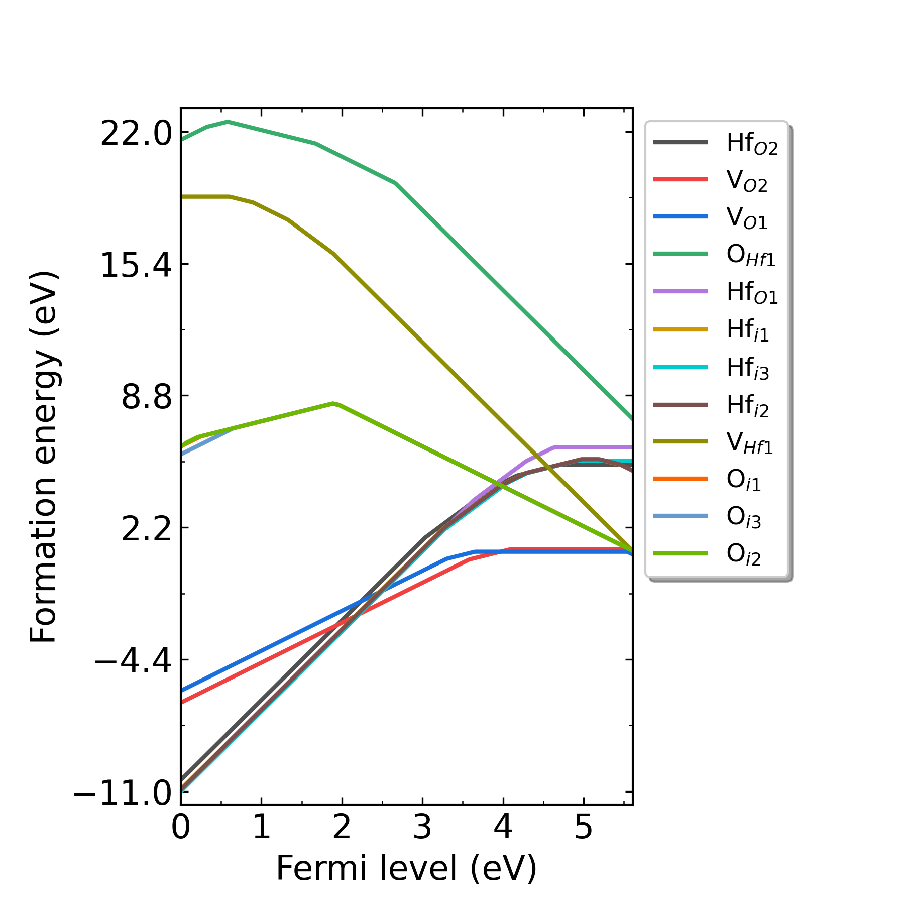turn to the directory HfO2 and execute the DEC module again with the command dasp 3 . The program will automatically judge the completed calculations, and recalculate the defect according to the redo.in .
The DEC module will carry out the calculations for the neutral and charged defect of Hf_O1, and calculate their formation energies.

Finally, DEC will automatically outputs the image of defect formation energy v.s. Fermi level by using all the corrected defect formation energies of HfO2 at two chemical potentials. As shown in below:

Fig: Formation energies of intrinsic defects in HfO2 as functions of Fermi level at p1 point (Hf-rich condition).

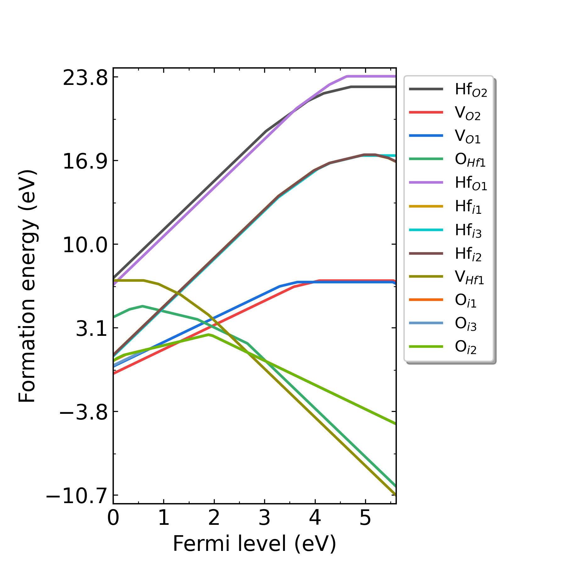
Fig: Formation energies of intrinsic defects in HfO2 as functions of Fermi level at p2 point (O-rich condition).

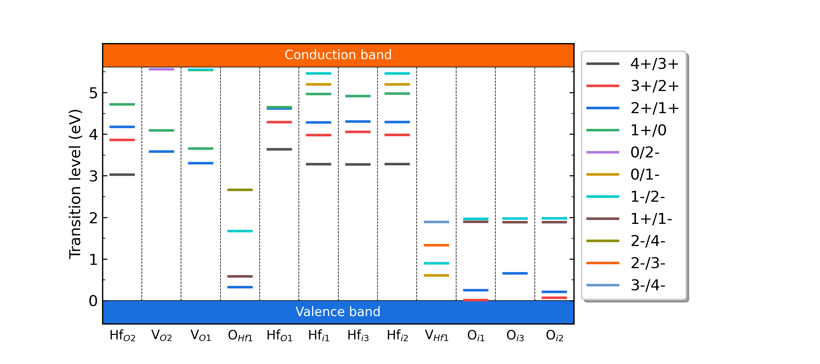
Meanwhile, the image of transition energy levels for each defect is also output, as shown in below:

Fig: The charge-state transition energy levels of intrinsic defects in HfO2.

5.2.4 DDC – defect density and Fermi level calculations¶

5.2.4.1 Run DDC module¶

After finishing the DEC module, return to the directory HfO2 and use the command dasp 4 to execute the DDC module. No additional operation is required while waiting for the program to complete.

5.2.4.2 Workflow of DDC module¶

Summarize the defect-related data:

Firstly, DDC module will judge which defects have been finished calculating based on the output of DEC module, and take all these defects into consideration in the DDC calculation. Then, DDC will search for the output information about each defect as formation energy, transition energy levels, and degeneracy factor. Finally, summarize all the data and write in the file DefectParams.txt .

4ddc.out is the log file of DDC module:

############ Collecting information from DEC ############
Read defect types from DEC calculation successfully.
Defects considered in DDC calculation: ['Hf_O2', 'V_O2', 'V_O1', 'O_Hf1', 'Hf_O1', 'Hf_i-1', 'Hf_i-3', 'Hf_i-2', 'V_Hf1', 'O_i-1', 'O_i-3', 'O_i-2']
Chemical potentials change from p1 to p2.
Calculate gq for defect in each charge state.
Calculate Nsites for Hf_O2: 5.708701e+22 cm^-3.
Calculate Nsites for V_O2: 5.708701e+22 cm^-3.
Calculate Nsites for V_O1: 5.708701e+22 cm^-3.
Calculate Nsites for O_Hf1: 2.854350e+22 cm^-3.
Calculate Nsites for Hf_O1: 5.708701e+22 cm^-3.
Calculate Nsites for Hf_i-1: 2.854350e+22 cm^-3.
Calculate Nsites for Hf_i-3: 2.854350e+22 cm^-3.
Calculate Nsites for Hf_i-2: 2.854350e+22 cm^-3.
Calculate Nsites for V_Hf1: 2.854350e+22 cm^-3.
Calculate Nsites for O_i-1: 2.854350e+22 cm^-3.
Calculate Nsites for O_i-3: 2.854350e+22 cm^-3.
Calculate Nsites for O_i-2: 2.854350e+22 cm^-3.
############ Collecting information from DEC ############

Below is the file DefectParams.txt :

800 300
2.950000 2.990000
5.611337
Hf_O2 5.708701e+22 1 4.714 2 4.444 1 4.25 2 3.944 1 x x x x x x x x 5.340000 22.964000
V_O2 5.708701e+22 1 4.089 2 3.835 1 x x x x 5.621 2 5.558 1 x x x x 1.106000 6.981000
V_O1 5.708701e+22 1 3.652 2 3.477 1 x x x x 5.539 2 5.542 1 x x x x 0.986000 6.861000
O_Hf1 2.854350e+22 1 0.79 2 0.557 1 x x x x 0.374 2 1.022 1 1.689 2 1.841 1 22.704000 5.080000
Hf_O1 5.708701e+22 1 4.646 2 4.631 1 4.517 2 4.296 1 x x x x x x x x 6.205000 23.830000
Hf_i-1 2.854350e+22 1 4.964 2 4.622 1 4.407 2 4.125 1 5.194 2 5.326 1 x x x x 5.601000 17.351000
Hf_i-3 2.854350e+22 1 4.914 2 4.608 1 4.423 2 4.135 1 x x x x x x x x 5.544000 17.294000
Hf_i-2 2.854350e+22 1 4.974 2 4.632 1 4.415 2 4.131 1 5.194 2 5.326 1 x x x x 5.614000 17.364000
V_Hf1 2.854350e+22 1 x x x x x x x x 0.606 2 0.751 1 0.944 2 1.18 1 18.743000 6.994000
O_i-1 2.854350e+22 1 2.09 2 1.17 1 0.784 2 x x 1.697 2 1.831 1 x x x x 8.596000 2.722000
O_i-3 2.854350e+22 1 2.093 2 1.374 1 0.814 2 x x 1.675 2 1.824 1 x x x x 8.606000 2.731000
O_i-2 2.854350e+22 1 2.095 2 1.153 1 0.791 2 x x 1.674 2 1.825 1 x x x x 8.606000 2.731000

Self-consistent calculation under growth temperature:

The DDC module will calculate the defect/dopant and carrier densities at the temperature T=800 K, and obtain the Fermi level by self-consistently under the charge neutralization condition.

Self-consistent calculation under working (measuring) temperature:

The DDC module will recalculate the defect/dopant and carrier densities at the temperature T=300 K, and re-obtain the Fermi level by self-consistently under the charge neutralization condition.

Output defect density:

DDC module will output three files in the directory CdTe/ddc: Fermi.dat , Carrier.dat , Defect_charge.dat , which can be plotted using Origin. In addition, DDC also can automatically generate image file density.png based on these three files, as follows:

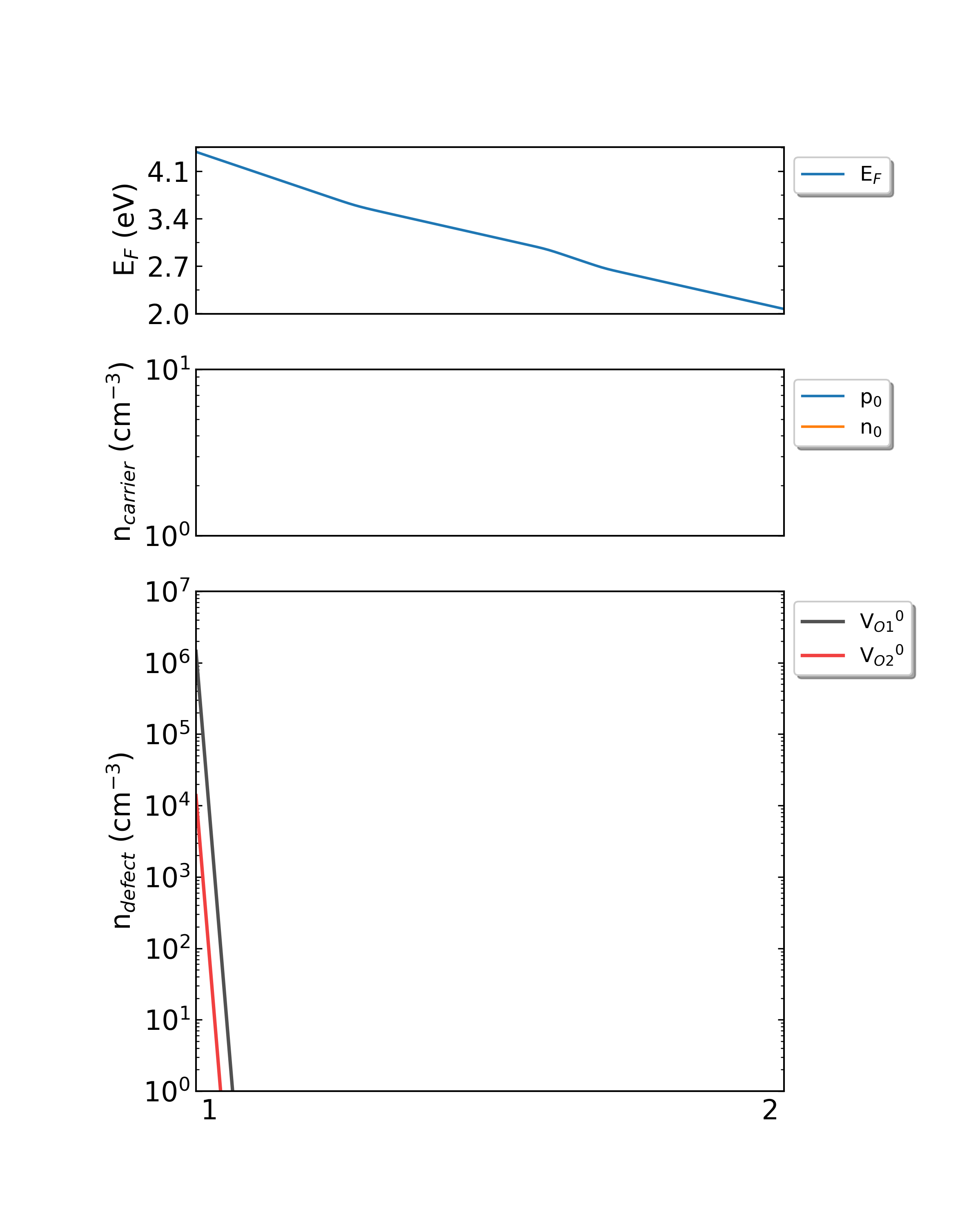
Fig: The Fermi level, electron and hole carrier densities, and defect densities in HfO2 as functions of the chemical potentials (from Hf-rich to O-rich) with a growth temperature is 300 K.

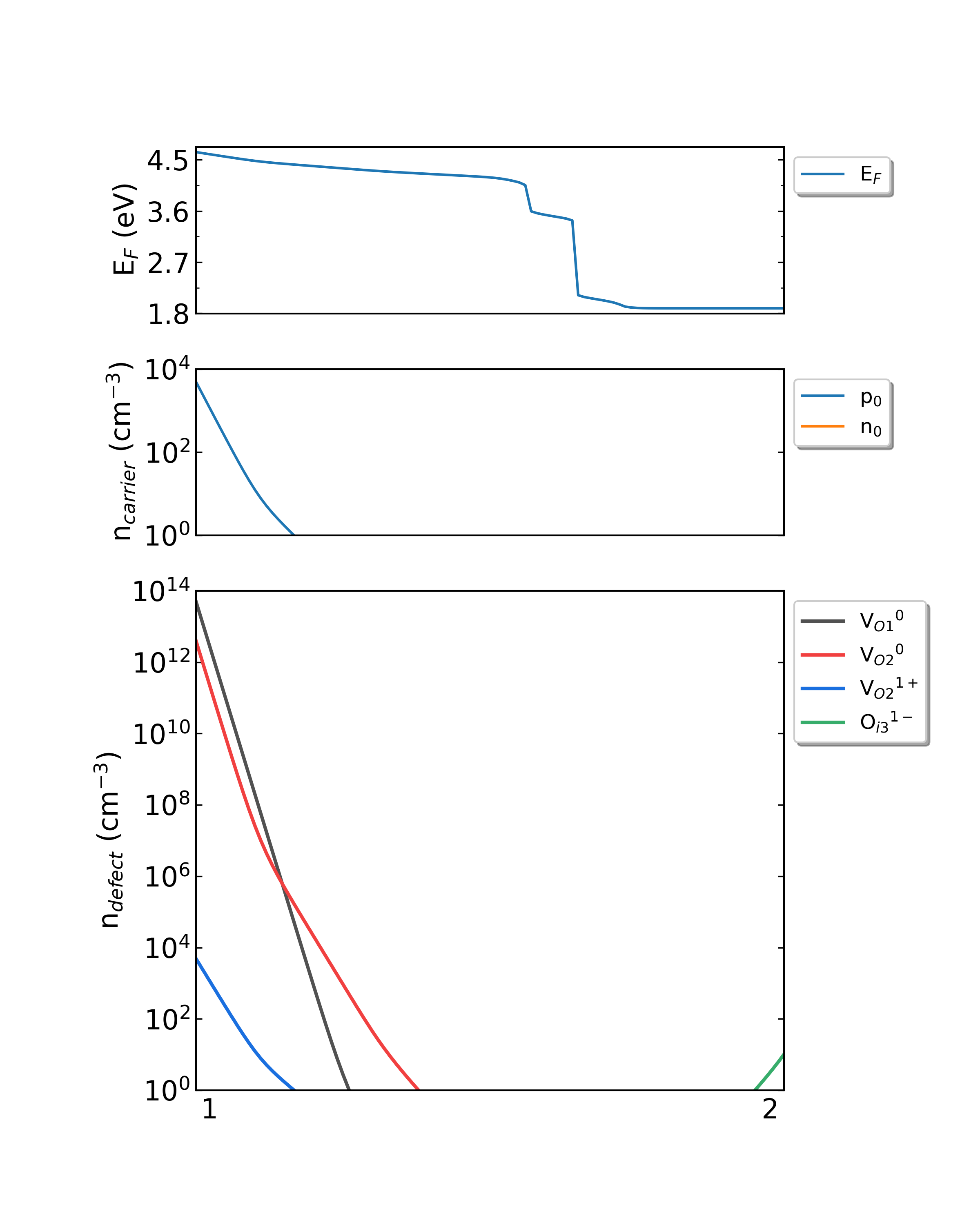
Fig: The Fermi level, electron and hole carrier densities, and defect densities in HfO2 as functions of the chemical potentials (from Hf-rich to O-rich) with a growth temperature is 550 K.

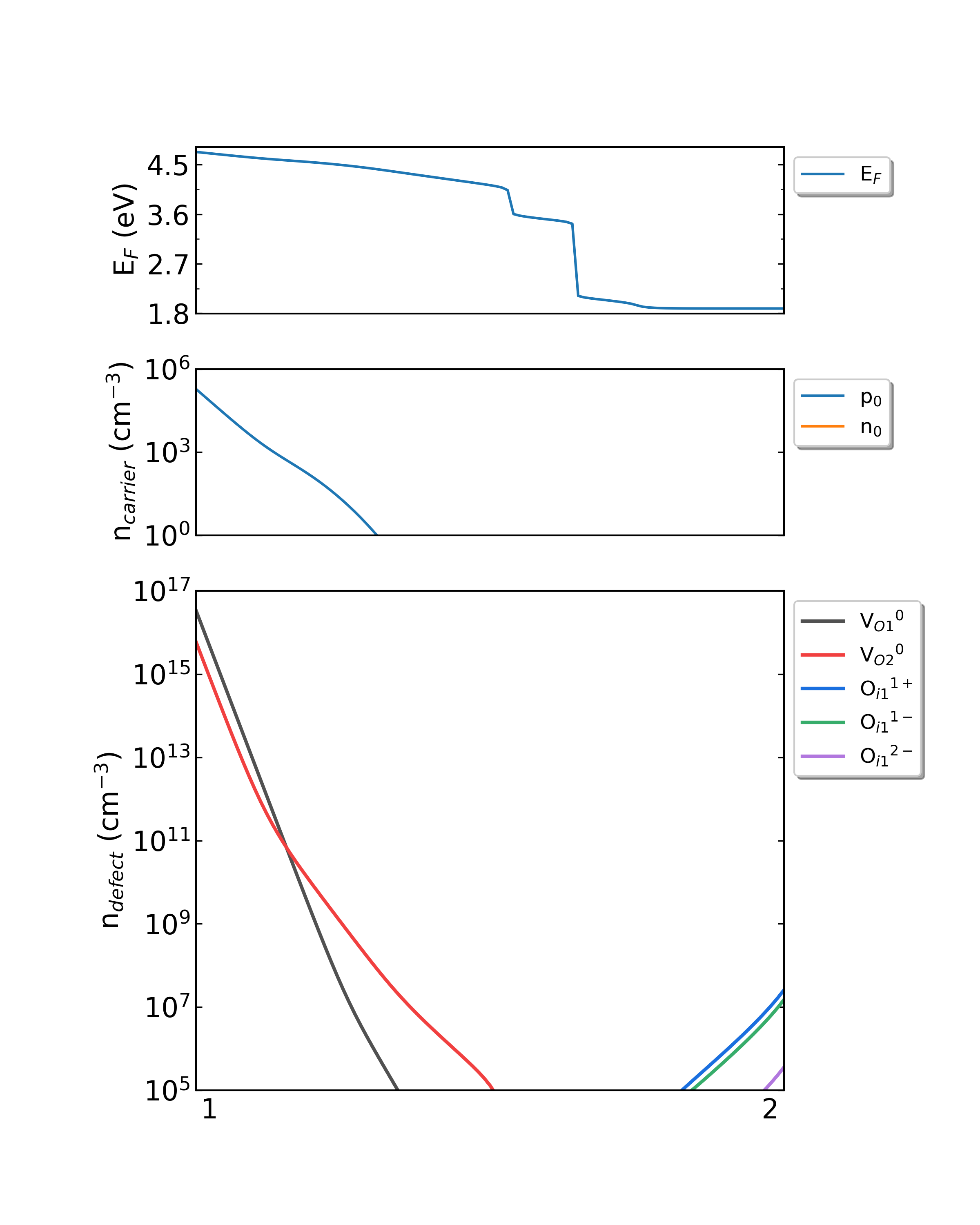
Fig: The Fermi level, electron and hole carrier densities, and defect densities in HfO2 as functions of the chemical potentials (from Hf-rich to O-rich) with a growth temperature is 800 K.

5.3 The Defect calculations for H-doped Ga2O3¶

Ga2O3 is a transparent conductive oxide material with a natural n-type conductivity and high optical transparency. It is used for various application fields, such as flat panel displays, touch panels and displays, top surface electrodes of solar cells, and solid-state light emitters.
Ga2O3 thin films and crystals show n-type conductivity without external doping, and the origin is controversial. Intrinsic defects and dopants both are possible inducements.
With the help of DASP software, the properties of the point defects and dopants can be systematically studied, and the mechanism of defects and dopants formation also can be explored to reveal the relationship between them and conductivity.

5.3.1 PREPARE — Prepares for calculation¶

5.3.1.1 POSCAR and dasp.in¶

Find the POSCAR for Ga2O3 from the Materials Project database, as follows:

Ga8 O12
1.0
           12.2299995422         0.0000000000         0.0000000000
            0.0000000000         3.0399999619         0.0000000000
           -1.3736609922         0.0000000000         5.6349851545
   Ga    O
    8   12
Direct
         0.158409998         0.500000000         0.314081997
         0.341589987         0.000000000         0.685917974
         0.089878000         0.000000000         0.794761002
         0.410122007         0.500000000         0.205238998
         0.658410013         0.000000000         0.314081997
         0.841589987         0.500000000         0.685917974
         0.589878023         0.500000000         0.794761002
         0.910121977         0.000000000         0.205238998
         0.495896995         0.000000000         0.256491005
         0.004103000         0.500000000         0.743508995
         0.173598006         0.000000000         0.564293981
         0.326402009         0.500000000         0.435705990
         0.336497009         0.500000000         0.891047001
         0.163503006         0.000000000         0.108952999
         0.995896995         0.500000000         0.256491005
         0.504103005         0.000000000         0.743508995
         0.673597991         0.500000000         0.564293981
         0.826402009         0.000000000         0.435705990
         0.836497009         0.000000000         0.891047001
         0.663502991         0.500000000         0.108952999

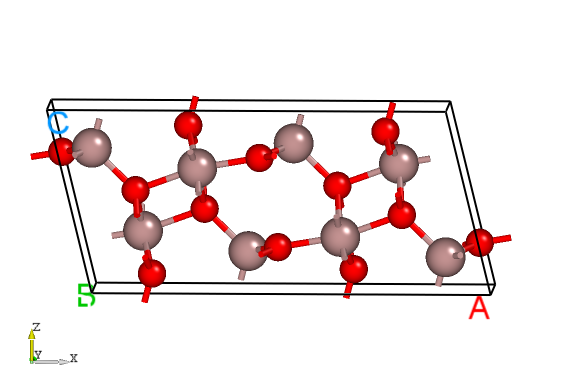
Taking it into the crystal visualization software, the structure can be seen as below:

The structure of Ga2O3.

Next, use VASP to optimize its lattice parameters or modify the lattice to match the experimental measurements. Users need to do it manually.

Write the required parameters in dasp.in :

############## Job Scheduling ##############
cluster = SLURM     # (job scheduling system)
node_number = 4         # (number of node)
core_per_node = 52      # (core per node)
queue = batch           # (name of queue/partition)
max_time = 24:00:00        # (maximum time for a single DFT calculation)
vasp_path_dec = /opt/vasp.5.4.4/bin/vasp_gam   #  (path of VASP)
vasp_path_tsc = /opt/vasp.5.4.4/bin/vasp_std
job_name = submit_job    # (name of script)
potcar_path = /opt/POT/potpaw_PBE    # (path of pseudopotentials)
max_job = 5

############## TSC Module ##############
database_api = ******************* # (str-list type)

############## DEC Module ##############
level = 2   # (level=1: PBE+PBE; level=2: PBE+HSE; level=3: HSE+HSE)
min_atom = 200
max_atom = 250
intrinsic = F   # (default: T)
doping = T   # (default: F)
impurity = H
correction = FNV   # (default: none)
epsilon = 10.8
Eg_real = 4.9   # (experimental band gap)

############## DDC Module ##############
ddc_temperature = 1124 300
ddc_mass = 0.23 2.90

Next, all the parameters listed in dasp.in will be described:

cluster = SLURM
# The system of the used cluster is SLURM.

node_number = 4
# 4 nodes are used for each calculation.

core_per_node = 52
# 52 cores are used for each node, so 4*52=208 cores are used in total for each calculation.

queue = batch
# The queue named “batch” is used to carry out calculations. Therefore, users need to make sure the queue name, nodes, and cores of clusters before configuring dasp.in.

max_time = 24:00:00        # (maximum time for a single DFT calculation)
# The maximum time allowed is 24 hours for a single DFT calculation and can be set arbitrarily.

vasp_path_dec = /opt/vasp.5.4.4/bin/vasp_gam   #  (path of VASP)
vasp_path_tsc = /opt/vasp.5.4.4/bin/vasp_std
# The VASP_std version is used for TSC calculations, and the VASP_gam version is used for DEC calculations.

job_name = submit_job    # (name of script)
# The submission script, named “ submit_job” and can be set arbitrarily.

potcar_path = /opt/POT/potpaw_PBE    # (path of pseudopotentials)
# path of pseudopotentials

max_job = 5
# the allowed maximum number of jobs at the same time

database_api = ******************* # (str-list type)
# using to visit the Materials Project database

level = 2   # (level=1: PBE+PBE; level=2: PBE+HSE; level=3: HSE+HSE)
# using GGA-PBE for structural relaxation and HSE to calculate the total energy

min_atom = 200
max_atom = 250
# The number of atoms within the generated supercell that we want is between 200 and 250, and as far as possible to make a=b=c and a⊥b⊥c.

intrinsic = F   # (default: T)
# Don’t generate intrinsic defects.

doping = T   # (default: F)
# Generate dopants.

impurity = H
# The doping element is H, and generate defects H_Ga, H_O, and H_i.

correction = FNV   # (default: none)
# The corrections for charged defect adopt FNV correction.

epsilon = 10.8
# The dielectric constant of Ga2O3 is 10.8.

Eg_real = 4.9   # (experimental band gap)
# The experimental band gap of Ga2O3 is about 4.9 eV, DASP will adjust AEXX in INCAR to make the band gap of the supercell without defect equal to 4.9 eV.

ddc_temperature = 1000 300
# the growth temperature set to 1000 K and the working temperature set to 300 K.

ddc_mass = 0.23 4.21
# electron effective mass set to 0.23 and hole effective mass set to 4.21.

5.3.1.2 Use DASP to generate the required input files¶

Create a new directory doping-Ga2O3, then prepare the files, POSCAR and dasp.in , mentioned above in the directory ./doping-Ga2O3/. Next, execute dasp 1 to start PREPARE module and no additional operation is needed thereafter. DASP will output file 1prepare.out to record the running log of the program.

5.3.1.3 Workflow of PREPARE module¶

Generate supercell:

Firstly, the program will automatically find the optimal supercell ( as far as possible to make a=b=c and a⊥b⊥c ) based on the parameters min_atom=200 and max_atom=250 and output POSCAR for the supercell. The following are the structure messages of Ga2O3 supercell POSCAR_nearlycube :

Cubic_cell
1.0
18.9887859181 0.0000000000 0.0000000000
-1.4600617135 9.0023673390 0.0000000000
0.7906182108 0.1282275357 14.7068652328
Ga O
96 144
Direct
0.1256845017 0.0418948339 0.5327255075
0.3743154982 0.2914384994 0.4672744924
0.2212487535 0.2404162511 0.3686292617
0.2787512464 0.0929170821 0.6313707382
0.8756845017 0.1252281672 0.2827255075
0.1243154982 0.0414384994 0.2172744924

...

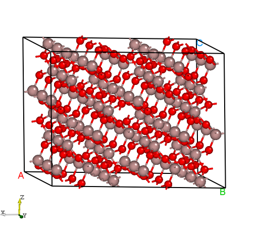
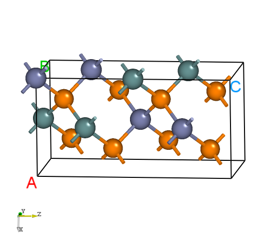
Taking it into the crystal visualization software, the supercell can be seen as below:

Fig: The structure of Ga2O3 supercell generated by DASP.

Madelung constant calculation:

Secondly, according to the generated supercell file, the program will execute Madelung constant calculation which describes the Coulomb interaction between charged defect and periodic image charge. (use for Lany-Zunger correction)

After finishing the above two steps calculation, the output of 1prepare.out is as follows:

############ Prepare Files module start ############

Read the structure file POSCAR you provided
Get the refined cell POSCAR_refined from POSCAR
Generate the nearlycube cell POSCAR_nearlycube from POSCAR
Generate job script through dasp.in parameters
Generate single-point KPOINTS
Generate pseudopotential file POTCAR through potcar_dir you set
Generate commonly used vasp input file INCAR
Start the madelung constant calculation
Generate the madelung calculation directory
Generate madelung calculation POSCAR
Generate madelung calculation POTCAR
Generate madelung calculation INCAR
Generate madelung calculation KPOINTS
Generate madelung calculation job script
Job 503.host5 submitted: /data2/home/chensy/zzn/doping-Ga2O3/dec/madelung/static
Succeed job 503.host5: /data2/home/chensy/zzn/doping-Ga2O3/dec/madelung/static
The madelung constant calculation completed
The madelung constant = 2.411

HSE exchange proportion calculation:

According to the generated supercell file, the program will perform HSE static calculations with AEXX=0.25 and AEXX=0.3 respectively to determine the value of AEXX which can make the obtained band gap match Eg_real = 4.9 based on the slope. If the calculated band gap with AEXX=0.25 or AEXX=0.3 is consistent with the set, the subsequent calculation for AEXX will not be performed. Therefore, after the calculation is completed, the contents in the directory doping-Ga2O3/dec/AEXX/ are as follows:

cd ./dec/AEXX
ls
0.25  0.3  0.3292780889291405  AEXX.list

It indicates that the band gap of the Ga2O3 supercell is 4.9 eV when AEXX=0.33 (two decimal places), and write this parameter into INCAR. Meanwhile, the log can be seen from 1prepare.out as follows:

Start the HSE parameter AEXX calculation
Job 507.host5 submitted: /data2/home/chensy/zzn/doping-Ga2O3/dec/AEXX/0.25/static
Succeed job 507.host5: /data2/home/chensy/zzn/doping-Ga2O3/dec/AEXX/0.25/static
Job 508.host5 submitted: /data2/home/chensy/zzn/doping-Ga2O3/dec/AEXX/0.3/static
Succeed job 508.host5: /data2/home/chensy/zzn/doping-Ga2O3/dec/AEXX/0.3/static
Job 509.host5 submitted: /data2/home/chensy/zzn/doping-Ga2O3/dec/AEXX/0.3292780889291405/static
Succeed job 509.host5: /data2/home/chensy/zzn/doping-Ga2O3/dec/AEXX/0.3292780889291405/static
The HSE parameter AEXX calculation completed
The HSE parameter AEXX = 0.33
level = 2: Generate PBE relax vasp input file INCAR-relax
level = 2: Generate HSE static vasp input file INCAR-static

Optimize the ionic position of the host supercell:

The last step in PREPARE module is to optimize the ionic position of the host supercell according to level=2 (i.e. PBE relax). The optimized file is POSCAR_final in the directory doping-Ga2O3/dec/relax. At the same time, the sign of the end of DASP operation can be seen in 1prepare.out , and it also tells us that we need to do the TSC module calculation in the next step.

Start the POSCAR_nearlycube relax calculation
Generate the POSCAR_nearlycube relax directory
Job 510.host5 submitted: /data2/home/chensy/zzn/doping-Ga2O3/dec/relax
Succeed job 510.host5: /data2/home/chensy/zzn/doping-Ga2O3/dec/relax
The POSCAR_nearlycube relax calculation completed
Get the final structure POSCAR_final

############ Prepare Files module end ############

DASP-PREPARE finished, please run DASP-TSC next

5.3.2 TSC – thermodynamic stability and chemical potential calculations¶

5.3.2.1 Run TSC module¶

The directory doping-Ga2O3/dec will be created when using the command dasp 1 to execute PREPARE module, and generate file 1prepare.out in this directory. After finishing the program, there has the corresponding completion flag in 1prepare.out . Then, enter the directory doping-Ga2O3/dec and confirm that the parameters in INCAR-relax and INCAR-static are feasible. (Users can modify INCAR, and DASP will make subsequent calculations based on the INCAR in this directory.)

Once confirm that the PREPARE module is finished, return to the directory doping-Ga2O3 and use the command dasp 2 to execute the TSC module. Similarly, the TSC module will create a directory named tsc under the directory doping-Ga2O3, which contains the output of the TSC program, including every calculation directory and the running log file 2tsc.out . No additional operation is required while waiting for the program to complete.

5.3.2.2 Workflow of TSC module¶

The total energy calculation of the host structure (the parameters are consistent with MP database):

TSC module will use the same input parameters (INCAR, KPOINTS, POTCAR) with the Materials Project database to perform structural relaxation and static calculation on the primitive cells given by the user. Therefore, the calculated total energy is comparable to that of the MP database. This step is to obtain the key hetero-phases that limit the stability of Ga2O3. In the directory, we can see:

cd tsc
cd Ga2O3/
ls
relaxation1  relaxation2  static

The running log also can be seen from the doping-Ga2O3/tsc/2tsc.out, that is, the steps such as generating input files, relaxation1, relaxation2, static and data extraction.

The judgement of key hetero-phases compounds:

The TSC module will search for all the secondary compounds that compete with Ga2O3 in the MP database. And compare the total energy of Ga2O3 calculated in the previous step with that of the hetero-phases extracted from the database to confirm Ga2O3 is thermodynamically stable.

Subsequently, the program will automatically download the key hetero-phase compounds that can limit the thermodynamic stability of H-doped Ga2O3. Only H and GaHO2 are considered in this case. The relevant information can be seen in 2tsc.out :

...
analysing the thermodynamic stability of Ga2O3.
The stability of Ga2O3 is: True.
key phases of Ga2O3 are: Ga O2 .
key phases of H doped Ga2O3 are: H2 GaHO2 .
analysing of Ga2O3 is done.
sub-module of tsc: 'auto thermodynamic calculation' ends successfully.
...

The total energy calculation of the host and hetero-phase compounds:

After the key hetero-phase compounds are confirmed, TSC will calculate the total energy of Ga2O3, GaHO2, and H2 by using the parameter (AEXX) obtained from PREPARE module. 2tsc.out is as follows:

...
Job 520.host5 submitted: /data2/home/chensy/zzn/doping-Ga2O3/tsc/GaHO2/static_recalc
Job 521.host5 submitted: /data2/home/chensy/zzn/doping-Ga2O3/tsc/H2/static_recalc
Succeed job  520.host5: /data2/home/chensy/zzn/doping-Ga2O3/tsc/GaHO2/static_recalc
Succeed job  521.host5: /data2/home/chensy/zzn/doping-Ga2O3/tsc/H2/static_recalc
...

The chemical potential calculation:

Calculating the formation energy and stable chemical potential region of H-doped Ga2O3 based on the calculated total energy. As Ga2O3 is a binary compound, TSC module will give the endpoint of two chemical potentials, i.e. Ga-rich and O-rich, and write them into dasp.in :

# The orders are consistent with the order of elements in POSCAR, i.e. the first column is Ga, the second column is O, and the third is the dopant H.
E_pure = -4.1294 -9.4157 1.0503
p1 = 0.0 -3.72 -4.9467
p2 = -5.5801 0.0 -6.8066

The output after the program is completed can be seen in 2tsc.out :

dir '2d-figures','3d-figures','ori_data_MP' ready.  analysing the thermodynamic stability of Ga2O3.
The stability of Ga2O3 is: True.
key phases of Ga2O3 are: Ga O2 .
key phases of H doped Ga2O3 are: H2 GaHO2 .
analysing of Ga2O3 is done.
sub-module of tsc: 'auto thermodynamic calculation' ends successfully.
--------------------------
DASP-TSC finished

For the ternary and multinary compounds, TSC module will output the image of the stable region and the chemical potential at the endpoint of the stable region.

5.3.3 DEC – the calculations of defect formation energy and transition energy level¶

5.3.3.1 Run DEC module¶

The directory doping-Ga2O3/tsc will be created when using the command dasp 2 to execute TSC module, and generate file 2tsc.out in this directory. After finishing the TSC module, there has the corresponding completion flag in 2tsc.out . Then, open the file dasp.in under the directory doping-Ga2O3/dasp.in to confirm the chemical potential already has been written.

Once confirm that the TSC module is finished, return to the directory doping-Ga2O3 and use the command dasp 3 to execute the DEC module. DEC will output relevant files in the generated directory dec in the first step, including the defect structures, directories, and the log file 3dec.out . No additional operation is required while waiting for the program to complete.

5.3.3.2 Workflow of DEC module¶

Generate defect structure:

Based on the parameters doping = T and impurity = H in dasp.in , DEC will generate the H-doped defects for Ga2O3, i.e. create the calculation directory doping-Ga2O3/dec/Doping-H, in which the structures and directories of substitutions H_Ga and H_O, and interstitial defect H_i. According to the crystal symmetry analysis, there have two inequivalent sites for Ga atom, and three inequivalent sites for O atom. Therefore, there will generate two different configurations for H_Ga and three configurations for H_O, while the number of configurations for H_i is depended on the input parameter set by users.

cd dec/Doping_H/
ls
Doping_H.list  H_Ga1  H_Ga2  H_i  H_O1  H_O2  H_O3  host

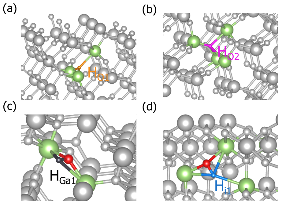
Take some defect structures to see in the visualization software, as shown in below:

Part of defect structures of H-doped Ga2O3 generated by DASP.

At the same time, the output of DEC module can be seen in 3dec.out as follows:

############ Neutral Defect module start ############
Make doping defect directory Doping_H
Generate host directory in Doping_H
Start generating neutral doping_H antisite defect
Generate neutral defect at: H_Ga1/initial_structure/q0
Generate neutral defect at: H_Ga2/initial_structure/q0
Generate neutral defect at: H_O1/initial_structure/q0
Generate neutral defect at: H_O2/initial_structure/q0
Generate neutral defect at: H_O3/initial_structure/q0
Neutral doping_H substitution defect generation completed
Start generating neutral doping_H interstitial defect
Generate neutral defect at: H_i/random1/initial_structure/q0
Generate neutral defect at: H_i/random2/initial_structure/q0
Generate neutral defect at: H_i/random3/initial_structure/q0
Generate neutral defect at: H_i/random4/initial_structure/q0
Generate neutral defect at: H_i/random5/initial_structure/q0
Generate neutral defect at: H_i/random6/initial_structure/q0
Neutral doping_H interstitial defect generation completed

############ Neutral Defect module end ############

It can be seen that the DEC module only creates the directories for all the neutral defects at this time.

Submit jobs for all defects with q=0:

After the structures and directories of neutral defects are generated, DEC module will call VASP to perform structural relaxation with PBE and total energy calculation with HSE (corresponds to the parameter level=2 in dasp.in ), this step may need a long time. Users can check the file 3dec.out at any time. The messages in 3dec.out are as follows:

Job 598.host5 submitted: /data2/home/chensy/zzn/doping-Ga2O3/H_Ga1/initial_structure/q0
Job 600.host5 submitted: /data2/home/chensy/zzn/doping-Ga2O3/H_Ga2/initial_structure/q0
Job 602.host5 submitted: /data2/home/chensy/zzn/doping-Ga2O3/H_O1/initial_structure/q0
Job 604.host5 submitted: /data2/home/chensy/zzn/doping-Ga2O3/H_O2/initial_structure/q0
Job 606.host5 submitted: /data2/home/chensy/zzn/doping-Ga2O3/H_O3/initial_structure/q0

...

Succeed job 602.host5: /data2/home/chensy/zzn/doping-Ga2O3/H_O1/initial_structure/q0
Succeed job 600.host5: /data2/home/chensy/zzn/doping-Ga2O3/H_Ga2/initial_structure/q0
Succeed job 598.host5: /data2/home/chensy/zzn/doping-Ga2O3/H_Ga1/initial_structure/q0
Succeed job 604.host5: /data2/home/chensy/zzn/doping-Ga2O3/H_O2/initial_structure/q0
Succeed job 606.host5: /data2/home/chensy/zzn/doping-Ga2O3/H_O3/initial_structure/q0

...

Generate calculation directories for the charged defects:

After finishing the calculations of all the neutral defects (except for interstitial defects with high energy), the program will judge the charge states of each defect and generate the corresponding directories and files for the charged defects based on the results of the neutral defects. A prompt will be given for those defects with calculation errors (undo, failed, and not converged) or without subsequent calculation (skip). The relevant information in 3dec.out is as follows:

############ Ionized Defect module start ############
Start generating ionized defects
Ionized defect path: /data2/home/chensy/zzn/doping-Ga2O3/H_O1/initial_structure/q+1
Ionized defect path: /data2/home/chensy/zzn/doping-Ga2O3/H_O1/initial_structure/q+2
Ionized defect path: /data2/home/chensy/zzn/doping-Ga2O3/H_O1/initial_structure/q+3
Ionized defect path: /data2/home/chensy/zzn/doping-Ga2O3/H_O1/initial_structure/q+4
Ionized defects generation completed
Start generating ionized defects
Ionized defect path: /data2/home/chensy/zzn/doping-Ga2O3/H_O2/initial_structure/q+1
Ionized defect path: /data2/home/chensy/zzn/doping-Ga2O3/H_O2/initial_structure/q+2
Ionized defect path: /data2/home/chensy/zzn/doping-Ga2O3/H_O2/initial_structure/q+3
Ionized defect path: /data2/home/chensy/zzn/doping-Ga2O3/H_O2/initial_structure/q+4
Ionized defects generation completed
The static calculation of /data2/home/chensy/zzn/doping-Ga2O3/H_i/random3/initial_structure/q0/static is skipped, skip ionized defect generation

...

Submit jobs for the defects with q≠0:

After the structures and directories of the charged defects are generated, DEC module will call VASP to perform structural relaxation with PBE and total energy calculation with HSE (corresponds to the parameter level=2 in dasp.in ). The waiting time needed in this step will be longer than that in 3.2.2. The messages in 3dec.out are as follows:

############ AutoRun - Ionized Defect module start ############
Job 659.host5 submitted: /data2/home/chensy/zzn/doping-Ga2O3/H_O1/initial_structure/q+2
Job 661.host5 submitted: /data2/home/chensy/zzn/doping-Ga2O3/H_O1/initial_structure/q+1
Job 663.host5 submitted: /data2/home/chensy/zzn/doping-Ga2O3/H_O1/initial_structure/q+3
Job 665.host5 submitted: /data2/home/chensy/zzn/doping-Ga2O3/H_O1/initial_structure/q-1
Job 667.host5 submitted: /data2/home/chensy/zzn/doping-Ga2O3/H_O2/initial_structure/q+2

...

Succeed job 659.host5: /data2/home/chensy/zzn/doping-Ga2O3/H_O1/initial_structure/q+2
Succeed job 661.host5: /data2/home/chensy/zzn/doping-Ga2O3/H_O1/initial_structure/q+1
Succeed job 663.host5: /data2/home/chensy/zzn/doping-Ga2O3/H_O1/initial_structure/q+3
Succeed job 665.host5: /data2/home/chensy/zzn/doping-Ga2O3/H_O1/initial_structure/q-1
Succeed job 667.host5: /data2/home/chensy/zzn/doping-Ga2O3/H_O2/initial_structure/q+2

...

Calculate the correction for the charged defects:

After finishing the calculations of all the charged defects (except for interstitial defects with high energy), DEC module will calculate the FNV correction (according to the parameter correction = FNV in dasp.in ), and then the formation energies and transition energy levels are also calculated. The specific data of the corrections and formation energies of different charge states of each defect are recorded in file 3dec.out :

...
The formation energy (neutral) of H_O1 at p1 is 1.84 eV
The formation energy (neutral) of H_O1 at p2 is 7.42 eV
The FNV correction (q = 2) E_correct =  -0.247 eV
The transition level (0/2+) above VBM: 2.627 eV
The FNV correction (q = 1) E_correct =  0.082 eV
The transition level (0/+) above VBM: 4.818 eV
The FNV correction (q = 3) E_correct =  -0.075 eV
The transition level (0/3+) above VBM: 1.739 eV
The FNV correction (q = -1) E_correct =  -0.056 eV
The transition level  (-/0) above VBM: 4.769 eV

...

The static calculation of /data2/home/chensy/zzn/doping-Ga2O3/dec/Doping_H/H_i/random3/initial_structure/q0/static is skipped, skip formation energy calculation

...

All the data related to formation energies and transition energy levels are also recorded in the file defect.log under each defect’s corresponding directories.

Output the image of formation energy:

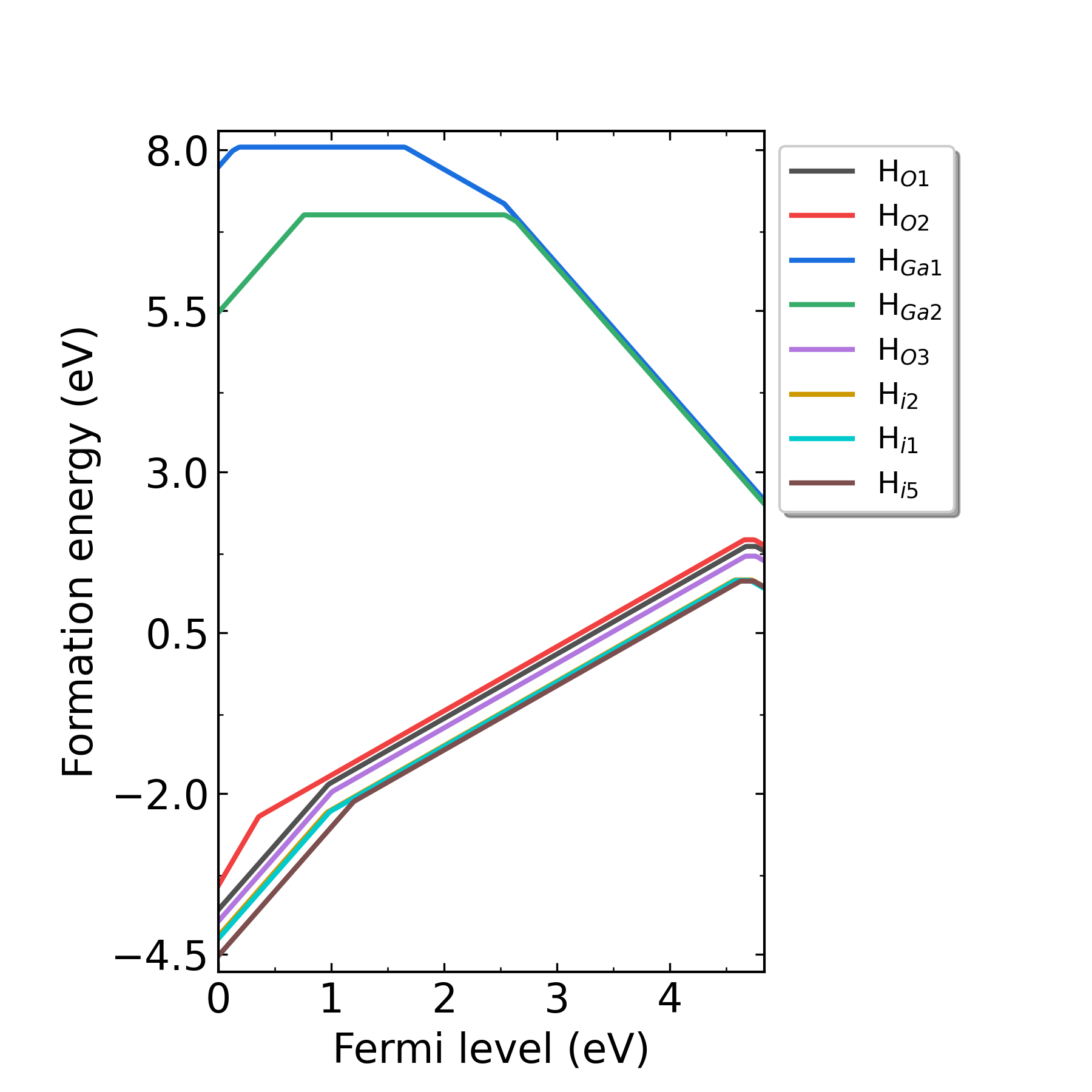
Finally, DEC will automatically output the image of defect formation energy v.s. Fermi level by using all the corrected defect formation energies of Ga2O3 at two chemical potentials. As shown in below:

Fig: Formation energies of H-related defects in H-doped Ga2O3 as functions of Fermi level at p1 point (Ga-rich condition).

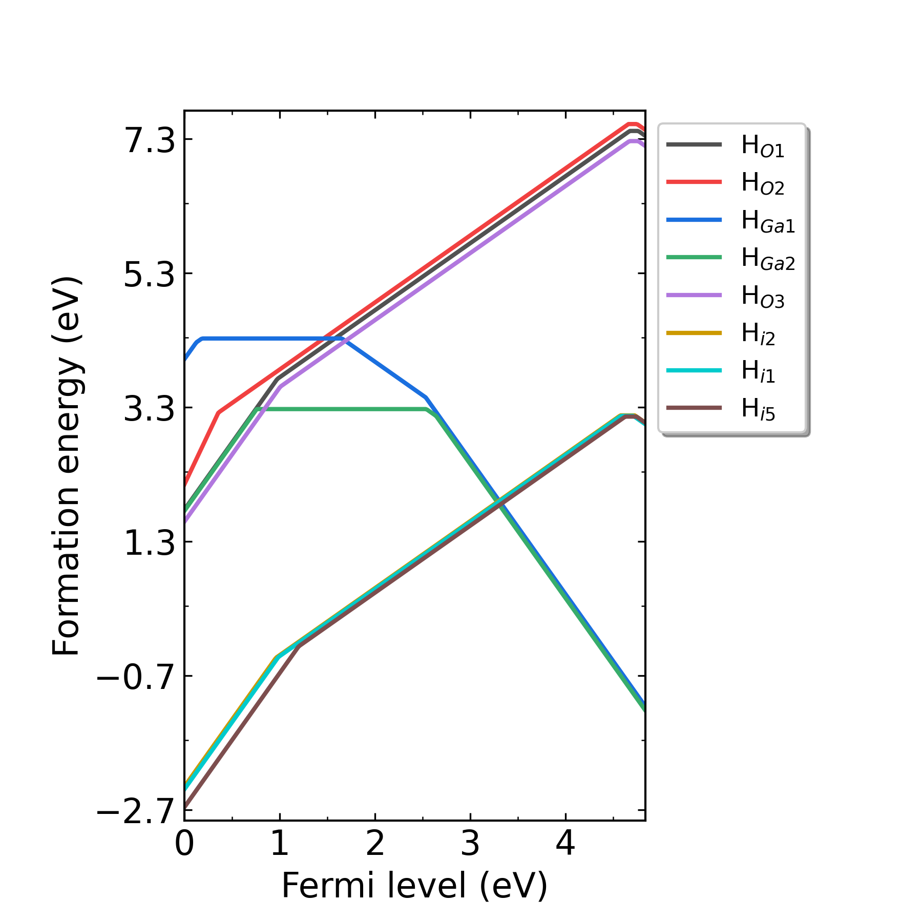
Fig: Formation energies of H-related defects in H-doped Ga2O3 as functions of Fermi level at p2 point (O-rich condition).

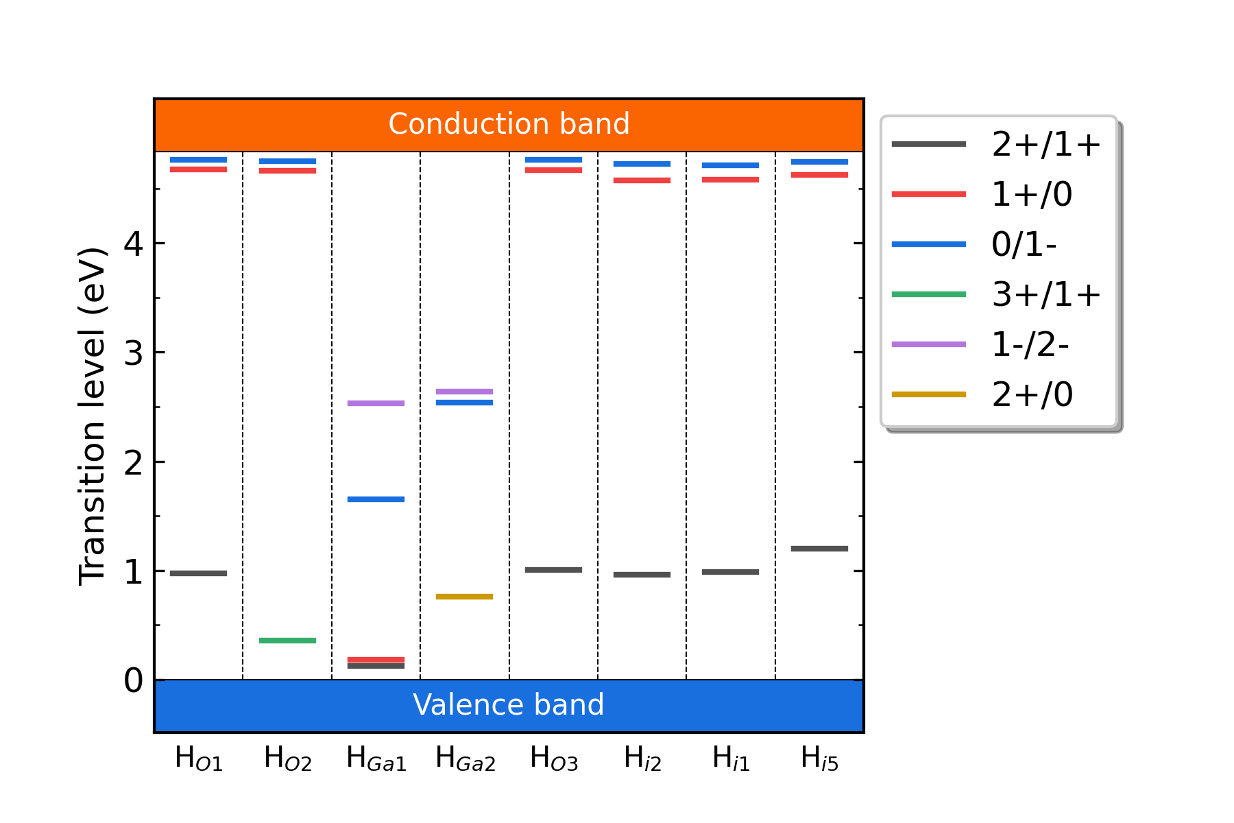
Meanwhile, the image of transition energy levels for each defect is also output, as shown in below:

Fig: The charge-state transition energy levels of H-related defects in H-doped Ga2O3.

5.3.4 DDC – defect density and Fermi level calculations¶

5.3.4.1 Run DDC module¶

After finishing the DEC module, return to the directory doping-Ga2O3 and use the command dasp 4 to execute the DDC module. No additional operation is required while waiting for the program to complete.

5.3.4.2 Workflow of DDC module¶

Summarize the defect-related data:

Firstly, DDC module will judge which defects have been finished calculating based on the output of DEC module, and take all these defects into consideration in the DDC calculation. Then, DDC will search for the output information about each defect as formation energy, transition energy levels, and degeneracy factor. Finally, summarize all the data and write in the file DefectParams.txt .

4ddc.out is the log file of DDC module:

############ Collecting information from DEC ############
Read defect types from DEC calculation successfully.
Defects considered in DDC calculation: ['H_O1', 'H_O2', 'H_Ga1', 'H_Ga2', 'H_O3', 'H_i-2', 'H_i-1', 'H_i-5']
Chemical potentials change from p1 to p2.
Calculate gq for defect in each charge state.
Calculate Nsites for H_O1: 5.727808e+22 cm^-3.
Calculate Nsites for H_O2: 5.727808e+22 cm^-3.
Calculate Nsites for H_Ga1: 3.818539e+22 cm^-3.
Calculate Nsites for H_Ga2: 3.818539e+22 cm^-3.
Calculate Nsites for H_O3: 5.727808e+22 cm^-3.
Calculate Nsites for H_i-2: 3.182116e+22 cm^-3.
Calculate Nsites for H_i-1: 3.182116e+22 cm^-3.
Calculate Nsites for H_i-5: 3.182116e+22 cm^-3.
############ Collecting information from DEC ############

Below is the file DefectParams.txt :

1000 300
0.230000 4.210000
4.836382
H_O1 5.727808e+22 2 4.818 1 2.627 2 1.739 1 x x 4.769 1 x x x x x x 1.840000 7.420000
H_O2 5.727808e+22 2 4.812 1 2.461 2 1.811 1 1.36 2 4.768 1 x x x x x x 1.942000 7.522000
H_Ga1 3.818539e+22 1 0.466 2 0.373 1 0.332 2 0.336 1 1.41 2 1.647 1 2.779 2 3.312 1 8.045000 4.325000
H_Ga2 3.818539e+22 1 0.857 2 0.756 1 0.571 2 0.374 1 2.307 2 2.163 1 3.112 2 3.554 1 6.993000 3.272000
H_O3 5.727808e+22 2 4.815 1 2.622 2 1.736 1 1.287 2 4.771 1 x x x x x x 1.688000 7.268000
H_i-2 3.182116e+22 2 4.738 1 2.571 2 1.708 1 1.266 2 4.733 1 x x x x x x 1.318000 3.178000
H_i-1 3.182116e+22 2 4.747 1 2.577 2 1.712 1 1.233 2 4.719 1 x x x x x x 1.311000 3.171000
H_i-5 3.182116e+22 2 4.779 1 2.581 2 1.592 1 1.23 2 4.741 1 x x x x x x 1.301000 3.160000

Self-consistent calculation under growth temperature:

The DDC module will calculate the dopant and carrier densities at the temperature T=1000 K, and obtain the Fermi level by self-consistently under the charge neutralization condition.

Self-consistent calculation under working (measuring) temperature:

The DDC module will recalculate the defect/dopant and carrier densities at the temperature T=300 K, and re-obtain the Fermi level by self-consistently under the charge neutralization condition.

Output defect density:

DDC module will output three files in the directory doping-Ga2O3/ddc: Fermi.dat , Carrier.dat , Defect_charge.dat , which can be plotted using Origin. In addition, DDC also can automatically generate image file density.png based on these three files, as follows:

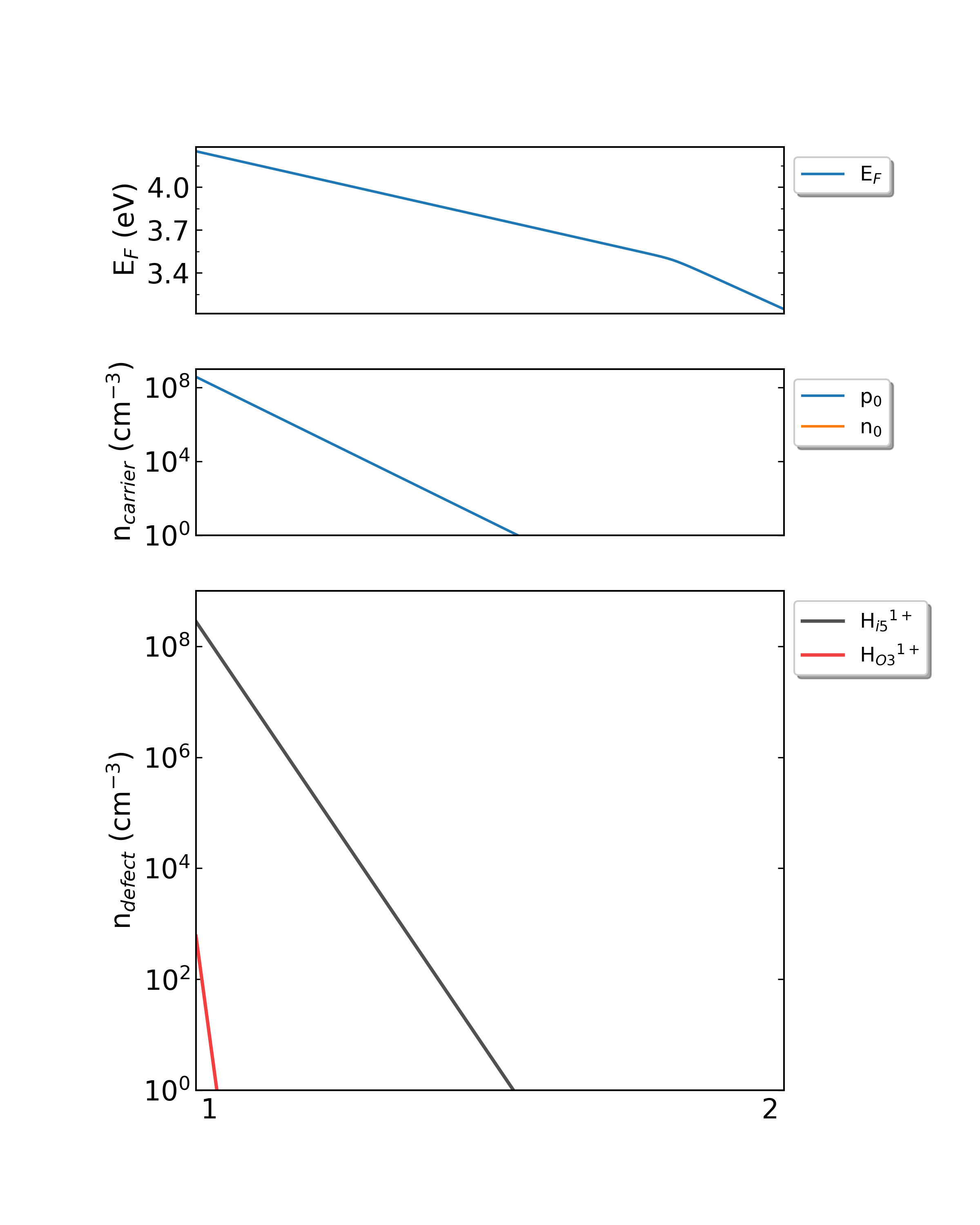
Fig: The Fermi level, electron and hole carrier densities, and defect densities in H-doped Ga2O3 as functions of the chemical potentials (from Ga-rich to O-rich) with a growth temperature is 300 K.

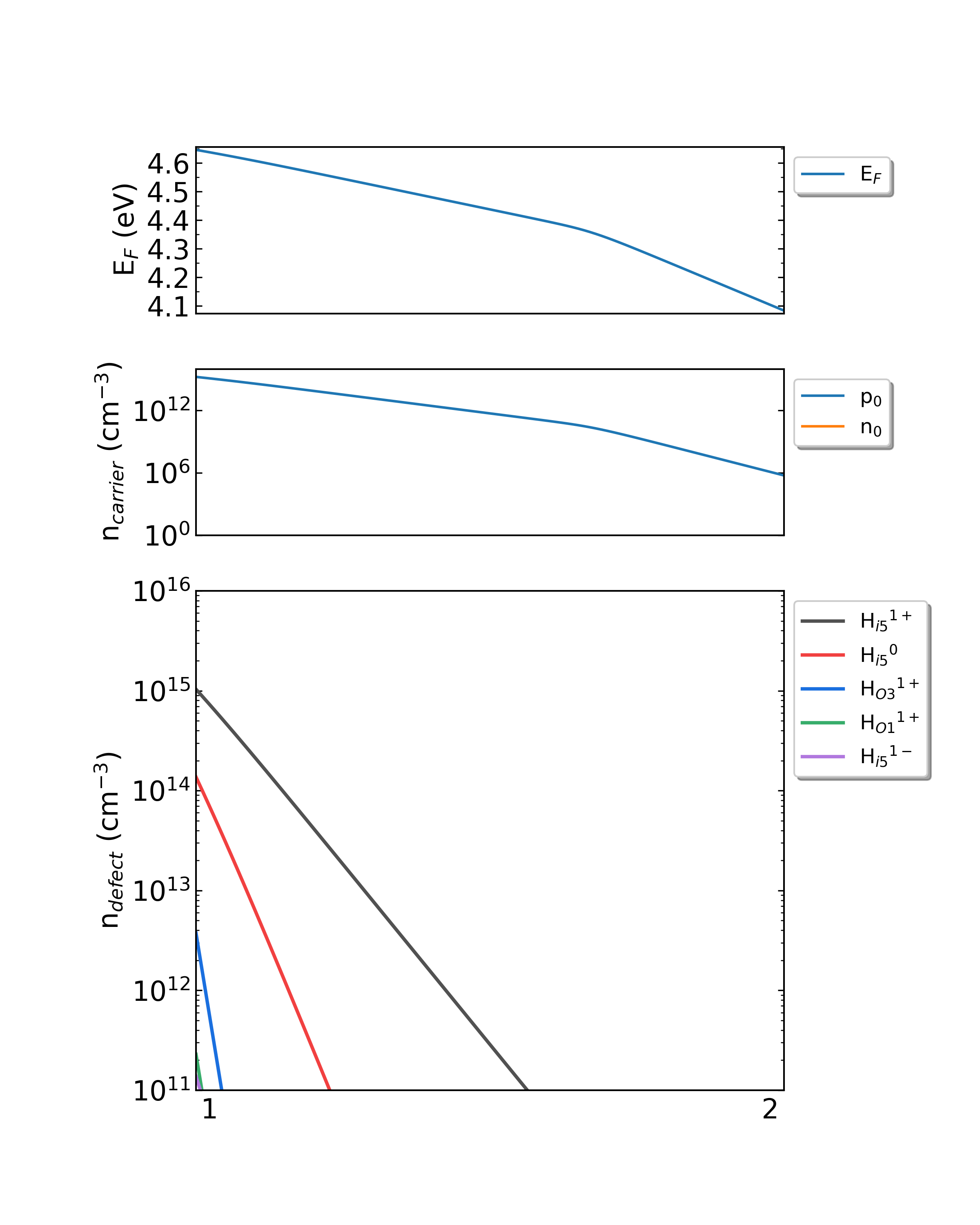
Fig: The Fermi level, electron and hole carrier densities, and defect densities in H-doped Ga2O3 as functions of the chemical potentials (from Ga-rich to O-rich) with a growth temperature is 650 K.

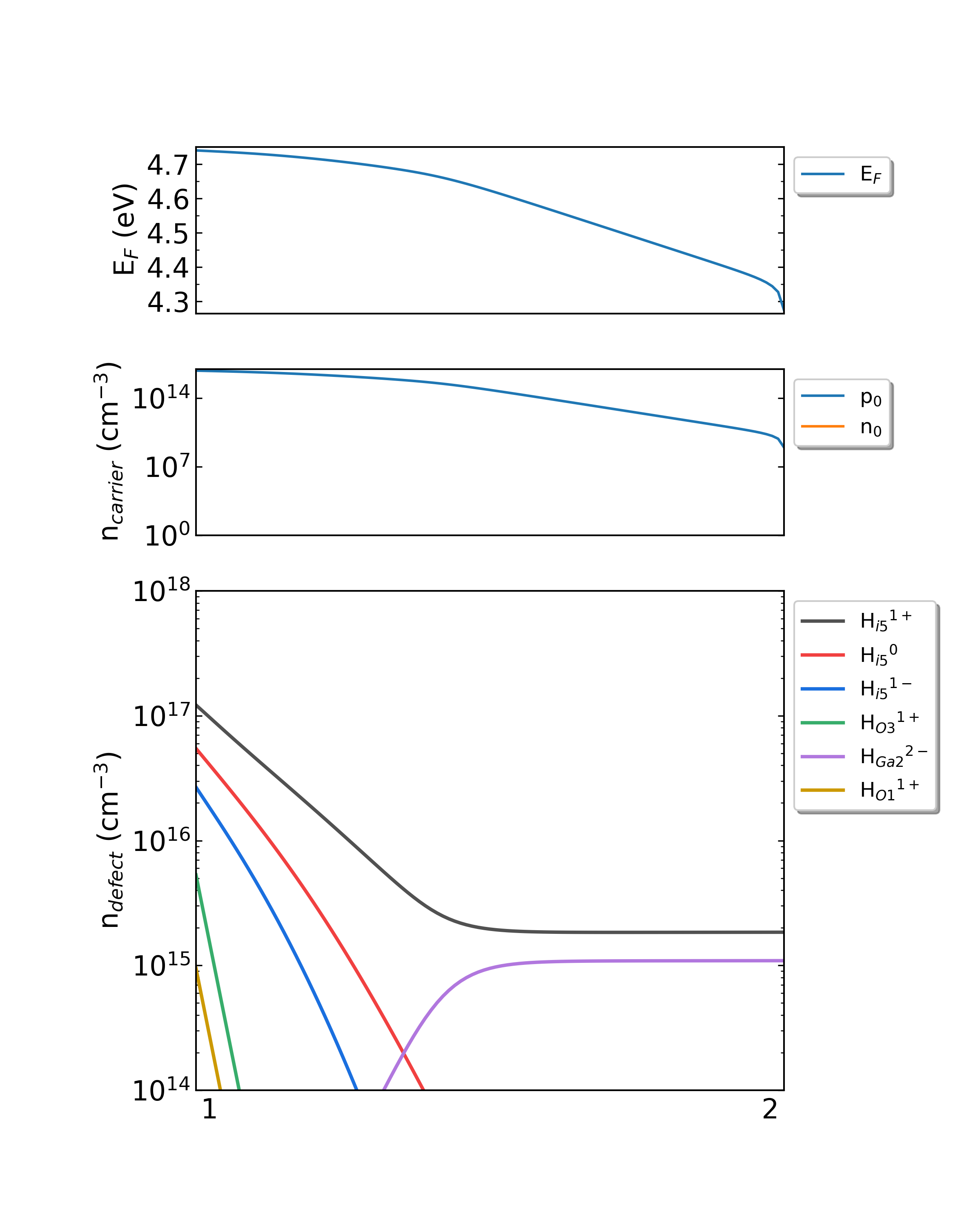
Fig: The Fermi level, electron and hole carrier densities, and defect densities in H-doped Ga2O3 as functions of the chemical potentials (from Ga-rich to O-rich) with a growth temperature is 1000 K.

5.4 The calculation of intrinsic defect in ZnGeP2¶

ZnGeP2 is a nonlinear optical material, and its application is limited by the existence of the optical absorption peaks in the band gap, which are believed to be related to point defects. Therefore, it is necessary to carry out a theoretical calculation of the point defect properties in ZnGeP2 and analyze the origin of its absorption peaks under different preparation environments.

The following is the example of using DASP to calculate intrinsic defects in ZnGeP2:

5.4.1 PREPARE — Prepares for calculation¶

5.4.1.1 POSCAR and dasp.in¶

Find the POSCAR for ZnGeP2, and use VASP to optimize its lattice parameters or modify the lattice to match the experimental measurements (Users need to do it manually). The information is as follows:

Zn4 Ge4 P8
0
468                0.0000000000         0.0000000000
0000000000         5.468                0.0000000000
0000000000         0.0000000000         10.745
Zn   Ge    P
  4    8
Direct
000000000         0.500000000         0.250000000
000000000         0.000000000         0.000000000
500000000         0.000000000         0.750000000
500000000         0.500000000         0.500000000
500000000         0.000000000         0.250000000
500000000         0.500000000         0.000000000
000000000         0.500000000         0.750000000
000000000         0.000000000         0.500000000
250000000         0.754127026         0.375000000
745872974         0.750000000         0.125000000
254126996         0.250000000         0.125000000
750000000         0.245873004         0.375000000
750000000         0.254126996         0.875000000
245873004         0.250000000         0.625000000
754127026         0.750000000         0.625000000
250000000         0.745872974         0.875000000

Using the crystal visualization software, the structure is shown in below:

The structure of ZnGeP2.

Write the required parameters in dasp.in :

############## Job Scheduling ##############
cluster = SLURM     # (job scheduling system)
node_number = 4         # (number of node)
core_per_node = 32      # (core per node)
queue = normal           # (name of queue/partition)
max_time = 24:00:00        # (maximum time for a single DFT calculation)
vasp_path_dec = /opt/vasp.5.4.4/bin/vasp_gam   #  (path of VASP)
vasp_path_tsc = /opt/vasp.5.4.4/bin/vasp_std
vasp_path_cdc=/opt/vasp-optics/bin/vasp_gam
job_name = submit_job    # (name of script)
potcar_path = /opt/POT/potpaw_PBE    # (path of pseudopotentials)
max_job = 5

############## TSC Module ##############
database_api = ******************* # (str-list type)

############## DEC Module ##############
level = 2   # (level=1: PBE+PBE; level=2: PBE+HSE; level=3: HSE+HSE)
min_atom = 180
max_atom = 200
intrinsic = T   # (default: T)
correction = FNV   # (default: none)
epsilon = 12.3
Eg_real = 2.06   # (experimental band gap)

############## DDC Module ##############
ddc_temperature = 1300 300
ddc_mass = 0.36 0.54
ddc_path = 1 2

############## CDC Module ###############
cdc_defect = Ge_Zn1
cdc_job = pl / radiative_rate
cdc_charge = 0 1
cdc_band = 864 865
cdc_temperature = 300
spin_channel = 2
refractive_index = 2.38

Next, all the parameters listed in dasp.in will be described:

cluster = SLURM
# The system of the used cluster is SLURM

node_number = 4
# 4 nodes are used for each calculation.

core_per_node = 32
# 32 cores are used for each node, so 4*32=128 cores are used in total for each calculation.

queue = normal
# The queue named “normal” is used to carry out calculations. Therefore, users need to make sure the queue name, nodes, and cores of clusters before configuring dasp.in.

max_time = 24:00:00        # (maximum time for a single DFT calculation)
# The queue named “normal” is used to carry out calculations. Therefore, users need to make sure the queue name, nodes, and cores of clusters before configuring dasp.in.

vasp_path_dec = /opt/vasp.5.4.4/bin/vasp_gam   #  (path of VASP)
vasp_path_tsc = /opt/vasp.5.4.4/bin/vasp_std
vasp_path_cdc = /opt/vasp-optics/bin/vasp_gam
# The VASP_std version is used for TSC calculations, and the VASP_gam version is used for DEC calculations. the VASP_gam version is specified in CDC calculation to calculate the carrier transition matrix element.

job_name = submit_job    # (name of script)
# The submission script, named “ submit_job” and can be set arbitrarily.

potcar_path = /opt/POT/potpaw_PBE    # (path of pseudopotentials)
# path of pseudopotentials

max_job = 5
# the allowed maximum number of jobs at the same time

database_api = ******************* # (str-list type)
# using to visit the Materials Project database

level = 2   # (level=1: PBE+PBE; level=2: PBE+HSE; level=3: HSE+HSE)
# using to visit the Materials Project database

min_atom = 180
max_atom = 200
# The number of atoms within the generated supercell that we want is between 180 and 200, and as far as possible to make a=b=c and a⊥b⊥c.

intrinsic = T   # (default: T)
# Generate intrinsic defects, V_Zn, V_Ge,V_P, Zn_Ge, Zn_P, Ge_Zn, Ge_P, P_Zn, P_Ge, Zn_i, Ge_i, and P_i.i

correction = FNV   # (default: none)
# The corrections for charged defect adopt FNV correction.

epsilon = 12.3
# The dielectric constant of ZnGeP2 is 12.3.

Eg_real = 2.06   # (experimental band gap)
# The experimental band gap of ZnGeP2 is about 2.06 eV, DASP will adjust AEXX in INCAR to make the band gap of the supercell without defect equal to 2.06 eV.

ddc_temperature = 1300 300
# the growth temperature set to 1300 K and the working temperature set to 300 K.

ddc_mass = 0.36 0.54
# electron effective mass set to 0.36 and hole effective mass set to 0.54.

ddc_path = 1 2
# set

cdc_defect = Ge_Zn1
# calculate the relevant properties of Ge_Zn1

cdc_job = pl / radiative_rate
# calculate the PL spectrum or radiative capture coefficient

cdc_charge = 0 1
# The defect state changes from the neutral state to the ionized state with +q, which is a hole transition.

cdc_band = 864 865
# hole transition, a hole transfer to the defect state from the valence band maximum, i.e. from the 864th band transfer to the 865th band.

cdc_temperature = 300
# calculate the defect properties at 300K in CDC module

spin_channel = 2
# The spin of the carrier is spin down.

refractive_index = 2.38
# The refractive index of ZnGeP2 is 2.38

5.4.1.2 Use DASP to generate the required input files¶

Create a new directory ZnGeP2, then prepare the files, POSCAR and dasp.in , mentioned above in the directory ./ZnGeP2/. Next, execute dasp 1 to start PREPARE module and no additional operation is needed thereafter. DASP will output file 1prepare.out to record the running log of the module.

5.4.1.3 Workflow of PREPARE module¶

Generate supercell:

Firstly, the program will automatically find the optimal supercell ( as far as possible to make a=b=c and a⊥b⊥c ) based on the parameters min_atom=180 and max_atom=200 and output POSCAR for the supercell. The following are the structure messages of supercell POSCAR_nearlycube expanded by ZnGeP2 primitive cell.

Cubic_cell
1.0
16.4040000000 0.0000000000 0.0000000000
0.0000000000 15.3313770093 0.0000000000
0.0000000000 0.2701043094 15.3289975100
Zn Ge P
48 48 96
Direct
0.0000000000 1.0000000000 0.2500000000
0.0000000000 0.0000000000 0.0000000000
0.1666666666 0.6250000000 0.3750000000
0.1666666666 0.8750000000 0.3750000000
...

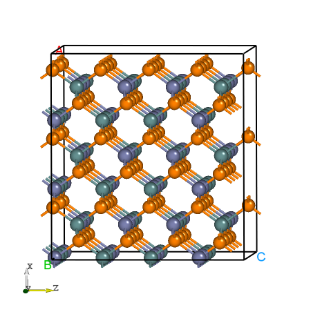
The supercell generated by DASP is shown in below:

Fig: The structure of ZnGeP2 supercell.

Madelung constant calculation:

Secondly, according to the generated supercell, the program will execute Madelung constant calculation which describes the Coulomb interaction between charged defect and periodic image charge. (use for Lany-Zunger correction)

After finishing the above two steps calculation, the output of 1prepare.out is as follows (**** indicates the job ID of the calculation):

############ Prepare Files module start ############

Read the structure file POSCAR you provided
Get the refined cell POSCAR_refined from POSCAR
Generate the nearlycube cell POSCAR_nearlycube from POSCAR
Generate job script through dasp.in parameters
Generate single-point KPOINTS
Generate pseudopotential file POTCAR through potcar_dir you set
Generate commonly used vasp input file INCAR
Start the madelung constant calculation
Generate the madelung calculation directory
Generate madelung calculation POSCAR
Generate madelung calculation POTCAR
Generate madelung calculation INCAR
Generate madelung calculation KPOINTS
Generate madelung calculation job script
Job ******** submitted: /home/test/ZnGeP2/dec/madelung/static
Succeed job ********: /home/test/ZnGeP2/dec/madelung/static
The madelung constant calculation completed
The madelung constant = 2.833

HSE exchange proportion calculation:

According to the generated supercell, the program will perform HSE static calculations with AEXX=0.25 and AEXX=0.3 respectively to determine the value of AEXX which can make the obtained band gap match Eg_real = 2.06 based on the slope. Therefore, after those calculations are completed, the contents in the directory ZnGeP2/dec/AEXX/ are as follows:

cd ./dec/AEXX
ls
0.25  0.26795555051593156  0.3  AEXX.list

It indicates that the band gap of the CdTe supercell is 2.06 eV when AEXX=0.27 (two decimal places), and write this parameter into INCAR . Meanwhile, the log can be seen from 1prepare.out as follows (**** indicates the job ID of the calculation):

Start the HSE parameter AEXX calculation
Job ******** submitted: /home/test/ZnGeP2/dec/AEXX/0.25/static
Job ******** submitted: /home/test/ZnGeP2/dec/AEXX/0.3/static
Succeed job ********: /home/test/ZnGeP2/dec/AEXX/0.25/static
Succeed job ********: /home/test/ZnGeP2/dec/AEXX/0.3/static
Job ******** submitted: /home/test/ZnGeP2/dec/AEXX/0.26795555051593156/static
Succeed job ********: /home/test/ZnGeP2/dec/AEXX/0.26795555051593156/static
The HSE parameter AEXX calculation completed
The HSE parameter AEXX = 0.27
level = 2: Generate PBE relax vasp input file INCAR-relax
level = 2: Generate HSE static vasp input file INCAR-static

Optimize the ionic position of the host supercell:

The last step in PREPARE module is to optimize the ionic position of the host supercell according to level=2 (PBE relax). The optimized file is POSCAR_final in the directory ZnGeP2/dec/relax. At the same time, the sign of the end of DASP operation can be seen in 1prepare.out , and it also tells us that we need to do the TSC module calculation in the next step (**** indicates the job ID of the calculation).

Start the POSCAR_nearlycube relax calculation
Generate the POSCAR_nearlycube relax directory
Job ******** submitted: /home/test/ZnGeP2/dec/relax
Succeed job ********: /home/test/ZnGeP2/dec/relax
The POSCAR_nearlycube relax calculation completed
Get the final structure POSCAR_final

############ Prepare Files module end ############

DASP-PREPARE finished, please run DASP-TSC next

5.4.2 TSC – thermodynamic stability and chemical potential calculations¶

5.4.2.1 Run TSC module¶

The directory ZnGeP2/dec will be created when using the command dasp 1 to execute PREPARE module, and generate file 1prepare.out in this directory. After finishing the program, there has the corresponding completion flag in 1prepare.out . Then, enter the directory ZnGeP2/dec and confirm that the parameters in INCAR-relax and INCAR-static are feasible. (Users can modify INCAR, and DASP will make subsequent calculations based on the INCAR in this directory.)

Once confirm that the PREPARE module is finished, return to the directory ZnGeP2 and use the command dasp 2 to execute the TSC module. Similarly, the TSC module will create a directory named tsc under the directory ZnGeP2, in which contains the output of the TSC program, including every calculation directory and the running log file 2tsc.out . No additional operation is required while waiting for the program to complete.

5.4.2.2 Workflow of TSC module¶

The total energy calculation of the host structure (the parameters are consistent with MP database):

TSC module will use the same input parameters (INCAR, KPOINTS, POTCAR) with the Materials Project database to perform structural relaxation and static calculation on the primitive cells given by the user. Therefore, the calculated total energy is comparable to that of the MP database. This step is to obtain the key hetero-phases that limit the stability of ZnGeP2. In the directory, we can see:

cd tsc
cd ZnGeP2/
ls
relaxation1  relaxation2  static

The running log also can be seen from the ZnGeP2/tsc/2tsc.out, that is, the steps such as generating input files, relaxation1, relaxation2, static and data extraction.

The judgement of key hetero-phases compounds:

The TSC module will search for all the secondary compounds that compete with ZnGeP2 in the MP database. And compare the total energy of ZnGeP2 calculated in the previous step with that of the hetero-phases extracted from the database to confirm ZnGeP2 is thermodynamically stable.

Subsequently, the program will automatically download the key hetero-phases compounds that can limit the thermodynamic stability of ZnGeP2. Ge, P, Zn3P2, ZnP2, and Zn are considered in this case. The relevant information can be seen in 2tsc.out ：

...
analysing the thermodynamic stability of ZnGeP2.
key phases of ZnGeP2 are: Ge P Zn3P2 ZnP2 Zn .
file key_phases_info_recalc.yaml generated.
analysing of ZnGeP2 is done.
...

The total energy calculation of the host and hetero-phase compounds:

After the key hetero-phase compounds are confirmed, TSC will calculate the total energy of ZnGeP2, Ge, P, Zn3P2, ZnP2, and Zn by using the parameter (AEXX) obtained from PREPARE module. 2tsc.out is as follows:

...
Job ******** submitted: /home/test/ZnGeP2/tsc/ZnGeP2/static_recalc
Job ******** submitted: /home/test/ZnGeP2/tsc/Ge/static_recalc
Job ******** submitted: /home/test/ZnGeP2/tsc/P/static_recalc
Job ******** submitted: /home/test/ZnGeP2/tsc/Zn3P2/static_recalc
Job ******** submitted: /home/test/ZnGeP2/tsc/ZnP2/static_recalc
Job ******** submitted: /home/test/ZnGeP2/tsc/Zn/static_recalc
Succeed job  ********: /home/test/ZnGeP2/tsc/ZnGeP2/static_recalc
Succeed job  ********: /home/test/ZnGeP2/tsc/Ge/static_recalc
Succeed job  ********: /home/test/ZnGeP2/tsc/P/static_recalc
Succeed job  ********: /home/test/ZnGeP2/tsc/Zn3P2/static_recalc
Succeed job  ********: /home/test/ZnGeP2/tsc/Zn/static_recalc
Succeed job  ********: /home/test/ZnGeP2/tsc/ZnP2/static_recalc
...

The chemical potential calculation:

Calculating the formation energy and stable chemical potential region of ZnGeP2 based on the calculated total energy. As ZnGeP2 is a ternary compound, TSC module will give the endpoint of four chemical potentials, and write them into dasp.in ：

# The orders are consistent with the order of elements in POSCAR, i.e. the first column is Zn, the second column is Ge, and the third column is P.
E_pure = -2.0283 -5.9739 -7.3365
p1 = -0.1456 0.0 -0.4672
p2 = -1.08 0.0 0.0
p3 = -0.9207 -0.1593 0.0
p4 = -0.2252 -0.1593 -0.3478

The output after the program is completed can be seen in 2tsc.out ：

dir '2d-figures','3d-figures','ori_data_MP' ready.  try to read file: 'calc_list.yaml'.
analysing the thermodynamic stability of ZnGeP2.
key phases of ZnGeP2 are: Ge P Zn3P2 ZnP2 Zn .
analysing of ZnGeP2 is done.

DASP-TSC finished

For the ternary and multinary compounds, TSC module will output the image of the stable region and the chemical potential at the endpoint of the stable region. In this directory, it can be seen:

cd tsc
cd 2d-figures/
ls
fig-ZnGeP2.png  fig-ZnGeP2_recalc.png  stable_2d.out stable_recalc_2d.out

The four files under the directory ZnGeP2/tsc/2d-figures/ are the images of the stable region plotted during the two calculations and analyses, and the chemical potential at each endpoint in the images.

Check out the files stable_2d.out and fig-ZnGeP2.png . The horizontal and vertical coordinates of fig-ZnGeP2.png are the chemical potential of the elements marked in the figure, and the shaded area is the stable region of the host compound. Each line on the boundary is the chemical potential curve at the critical condition where the marked material can or can not form. This is the image output from the first calculation and analysis process.

     Ge       Zn        P
-------  -------  -------
-0.0999  -0.7457   0
0        -0.8457   0
0        -0.0484  -0.3986
-0.0999  -0.0983  -0.3237

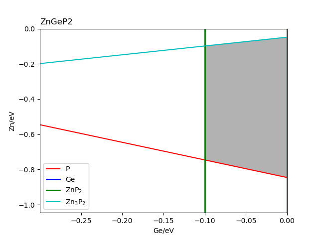
Fig: The stable chemical potential region of ZnGeP2. (comes from the MP database)

Check out the files stable_recalc_2d.out and fig-ZnGeP2_recalc.png . They are the image and data output from the second calculation and analysis process.

     Ge       Zn        P
-------  -------  -------
-0.1593  -0.9207   0
0        -1.08     0
0        -0.1456  -0.4672
-0.1593  -0.2252  -0.3478

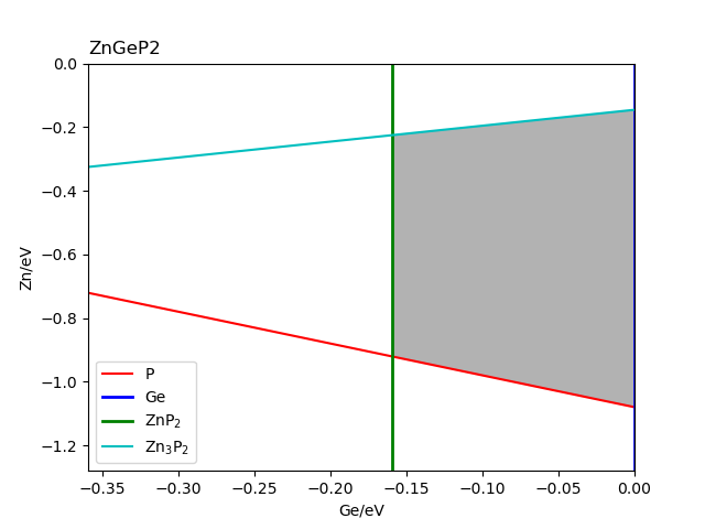
Fig: The stable chemical potential region of ZnGeP2. (comes from the DFT calculation)

5.4.3 DEC – the calculations of defect formation energy and transition energy level¶

5.4.3.1 Run DEC module¶

The directory ZnGeP2/tsc will be created when using the command dasp 2 to execute TSC module, and generate file 2tsc.out in this directory. After finishing the TSC module, there has the corresponding completion flag in 2tsc.out . Then, open the file dasp.in under the directory ZnGeP2/dasp.in to confirm the chemical potential already has been written.

Once confirm that the TSC module is finished, return to the directory ZnGeP2 and use the command dasp 3 to execute the DEC module. DEC will output relevant files in the generated directory dec in the first step, including the defect structures, directories, and the log file 3dec.out . No additional operation is required while waiting for the program to complete.

5.4.3.2 Workflow of DEC module¶

Generate defects structure:

In order to calculate the defect properties of ZnGeP2, the program will generate the directories and structures corresponding to the neutral defects that need to be calculated based on the user setting in dasp.in :

cd dec
cd Intrinsic_Defect
ls
Ge_i   Ge_Zn1  Intrinsic_Defect.list  P_i    V_Ge1  V_Zn1   Zn_i
Ge_P1  host    P_Ge1                  P_Zn1  V_P1   Zn_Ge1  Zn_P1

At the same time, the output of DEC module can be seen in 3dec.out as follows:

############ Neutral Defect module start ############
Make intrinsic defect directory Intrinsic_Defect
Generate host directory in Intrinsic_Defect
Start generating neutral vacancy defect
Generate neutral defect at: V_Zn1/initial_structure/q0
Generate neutral defect at: V_Ge1/initial_structure/q0
Generate neutral defect at: V_P1/initial_structure/q0
Neutral vacancy defect generation completed
Start generating neutral intrinsic antisite defect
Generate neutral defect at: Ge_Zn1/initial_structure/q0
Generate neutral defect at: P_Zn1/initial_structure/q0
Generate neutral defect at: Zn_Ge1/initial_structure/q0
Generate neutral defect at: P_Ge1/initial_structure/q0
Generate neutral defect at: Zn_P1/initial_structure/q0
Generate neutral defect at: Ge_P1/initial_structure/q0
Neutral intrinsic antisite defect generation completed
Start generating neutral intrinsic interstitial defect
Generate neutral defect at: Zn_i/random1/initial_structure/q0
Generate neutral defect at: Zn_i/random2/initial_structure/q0
...
Generate neutral defect at: Ge_i/random1/initial_structure/q0
Generate neutral defect at: Ge_i/random2/initial_structure/q0
...
Generate neutral defect at: P_i/random1/initial_structure/q0
Generate neutral defect at: P_i/random2/initial_structure/q0
...
Neutral intrinsic interstitial defect generation completed

############ Neutral Defect module end ############

Among the generated defect structures, part of antisite and possible interstitial defects is shown in below:

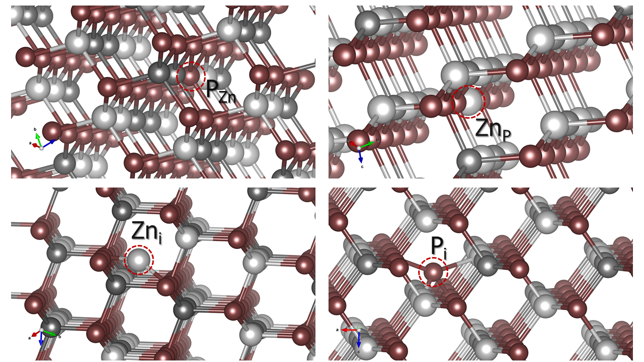
Part of defect structures of ZnGeP2.

Submit jobs for all defects with q=0:

After the structures and directories of neutral defects are created, DEC module will automatically supplement the files required for the calculations and submit jobs in turn, so that the number of jobs to be calculated at the same time does not exceed the value of max_job in dasp.in . The following logs can be seen in file 3dec.out :

############ AutoRun - Neutral Defect module start ############
Job ******** submitted: /data/home/test/Zn_Ge_P/DASP-test-0128/dec/Intrinsic_Defect/P_Zn1/initial_structure/q0
Job ******** submitted: /data/home/test/Zn_Ge_P/DASP-test-0128/dec/Intrinsic_Defect/Zn_P1/initial_structure/q0
Job ******** submitted: /data/home/test/Zn_Ge_P/DASP-test-0128/dec/Intrinsic_Defect/Ge_P1/initial_structure/q0
Job ******** submitted: /data/home/test/Zn_Ge_P/DASP-test-0128/dec/Intrinsic_Defect/P_Ge1/initial_structure/q0
Job ******** submitted: /data/home/test/Zn_Ge_P/DASP-test-0128/dec/Intrinsic_Defect/P_i/random3/initial_structure/q0
Succeed job ********: /data/home/test/Zn_Ge_P/DASP-test-0128/dec/Intrinsic_Defect/Zn_P1/initial_structure/q0
Job ******** submitted: /data/home/test/Zn_Ge_P/DASP-test-0128/dec/Intrinsic_Defect/P_i/random1/initial_structure/q0
Succeed job ********: /data/home/test/Zn_Ge_P/DASP-test-0128/dec/Intrinsic_Defect/Ge_P1/initial_structure/q0
...

############ AutoRun - Neutral Defect module end ############

Generate calculation directories for the charged defects:

After finishing the calculations of all the neutral defects, the program will judge the charge states of each defect and generate the corresponding directories and files for the charged defects based on the results of the neutral defects.

############ Ionized Defect module start ############
Start generating ionized defects
Ionized defect path: /data/home/test/Zn_Ge_P/DASP-test-0128/dec/Intrinsic_Defect/P_Zn1/initial_structure/q-4
Ionized defect path: /data/home/test/Zn_Ge_P/DASP-test-0128/dec/Intrinsic_Defect/P_Zn1/initial_structure/q-3
...
Ionized defects generation completed

############ Ionized Defect module end ############

Submit jobs for the defects with q≠0:

After the structures and directories of the charged defects are created, DEC module will automatically supplement the files required for the calculations and submit jobs in turn, so that the number of jobs to be calculated at the same time does not exceed the value of max_job in dasp.in . The following logs can be seen in file 3dec.out :

############ AutoRun - Ionized Defect module start ############
Job ******** submitted: /data/home/test/Zn_Ge_P/DASP-test-0128/dec/Intrinsic_Defect/P_Zn1/initial_structure/q-1
Job ******** submitted: /data/home/test/Zn_Ge_P/DASP-test-0128/dec/Intrinsic_Defect/P_Zn1/initial_structure/q-4
Job ******** submitted: /data/home/test/Zn_Ge_P/DASP-test-0128/dec/Intrinsic_Defect/P_Zn1/initial_structure/q-2
Job ******** submitted: /data/home/test/Zn_Ge_P/DASP-test-0128/dec/Intrinsic_Defect/P_Zn1/initial_structure/q+3
Job ******** submitted: /data/home/test/Zn_Ge_P/DASP-test-0128/dec/Intrinsic_Defect/P_Zn1/initial_structure/q-3
Succeed job ********: /data/home/test/Zn_Ge_P/DASP-test-0128/dec/Intrinsic_Defect/P_Zn1/initial_structure/q-1
Job ******** submitted: /data/home/test/Zn_Ge_P/DASP-test-0128/dec/Intrinsic_Defect/P_Zn1/initial_structure/q+1
...

############ AutoRun - Ionized Defect module end ############

Calculate the correction for the charged defects:

After finishing the calculations of all the charged defects, the program will calculate the formation energies and transition energy levels for each defect. The formation energies, band alignment, image charge correction (LZ/FNV), and the transition energy levels of each defect under different chemical potentials are recorded in the log file 3dec.out . There are four formation energies corresponding to the four chemical potentials at p1, p2, p3, and p4 of each element provided in file dasp.in . The following logs can be seen in file 3dec.out :

############ Formation Energy module start ############
Start the formation energy calculation

The formation energy (neutral) of P_Zn1 at p1 is 3.993075
The formation energy (neutral) of P_Zn1 at p2 is 2.591475
The formation energy (neutral) of P_Zn1 at p3 is 2.750775
The formation energy (neutral) of P_Zn1 at p4 is 3.794075
The FNV correction (q = -1) E_correct =  0.0859854 eV
The transition level  (-/0) above VBM: 1.3758
The FNV correction (q = -4) E_correct =  1.43843 eV
The transition level  (4-/0) above VBM: 2.0373
...

############ Formation Energy module end ############

Output the image of formation energy:

After the calculations of formation energy and transition energy level for each kind of defect are completed, DEC module will automatically output the image of defect formation energy and data under different chemical potential conditions, and save it in the directory /dec/Formation_Energy_Intrinsic_Defect/. As four values of the chemical potential of each element are provided in file dasp.in , there are also four images and corresponding data.

cd dec
cd Formation_Energy_Intrinsic_Defect/
ls
p1.dat  p1.png  p2.dat  p2.png  p3.dat  p3.png  p4.dat  p4.png

Users can plot manually based on the data file with .dat format, or refer to the image file with .png format automatically generated by the program. The following logs can be seen in file 3dec.out :

############ Plot Diagram module start ############
Start plotting the diagrams
Generate formation energy diagrams at p1: /data/home/test/Zn_Ge_P/DASP-test-0128/dec/Formation_Energy_Intrinsic_Defect/p1.dat
Generate formation energy diagrams at p2: /data/home/test/Zn_Ge_P/DASP-test-0128/dec/Formation_Energy_Intrinsic_Defect/p2.dat
Generate formation energy diagrams at p3: /data/home/test/Zn_Ge_P/DASP-test-0128/dec/Formation_Energy_Intrinsic_Defect/p3.dat
Generate formation energy diagrams at p4: /data/home/test/Zn_Ge_P/DASP-test-0128/dec/Formation_Energy_Intrinsic_Defect/p4.dat
Generate transition level diagram: /data/home/test/Zn_Ge_P/DASP-test-0128/dec/Transition_Level_Intrinsic_Defect/tl.dat
All diagrams completed

############ Plot Diagram module end ############

The four images automatically plotted by DEC module are shown in below:

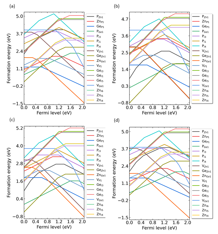
Fig: Formation energies of intrinsic defects in ZnGeP2 as functions of Fermi level under different chemical potentials: (a) p1, (b) p2, (c) p3, and (d) p4.

5.4.4 DDC – defect density and Fermi level calculations¶

5.4.4.1 Run DDC module¶

After finishing the DEC module, return to the directory ZnGeP2 and use the command dasp 4 to execute the DDC module. No additional operation is required while waiting for the program to complete.

5.4.4.2 Workflow of DDC module¶

Summarize the defect-related data:

Firstly, DDC module will judge which defects have been finished calculating based on the output of DEC module, and take all these defects into consideration in the DDC calculation. Then, DDC will search for the output information about each defect as formation energy, transition energy levels, and degeneracy factor. Finally, summarize all the data and write in the file DefectParams.txt .

4ddc.out is the log file of DDC module:

############ Collecting information from DEC ############
Read defect types from DEC calculation successfully.
Defects considered in DDC calculation: ['P_Zn1', 'Zn_P1', 'Ge_P1', 'P_Ge1', 'P_i-3', 'P_i-1', 'P_i-4', 'V_Zn1', 'Ge_Zn1', 'Zn_Ge1', 'V_P1', 'Ge_i-3', 'Ge_i-1', 'Ge_i-5', 'V_Ge1', 'Zn_i-6', 'Zn_i-5', 'Zn_i-4']
Chemical potentials change from p1 to p2.
Calculate gq for defect in each charge state.
Calculate Nsites for P_Zn1: 1.245078e+22 cm^-3.
Calculate Nsites for Zn_P1: 2.490156e+22 cm^-3.
Calculate Nsites for Ge_P1: 2.490156e+22 cm^-3.
Calculate Nsites for P_Ge1: 1.245078e+22 cm^-3.
Calculate Nsites for P_i-3: 1.660104e+22 cm^-3.
Calculate Nsites for P_i-1: 1.660104e+22 cm^-3.
...
############ Collecting information from DEC ############

Below is the file DefectParams.txt :

1300 300
0.360000 0.540000
2.067143
P_Zn1 1.245078e+22 2 1.0959 1 0.7854 2 0.602 1 0.3478 2 1.3758 1 1.8193 2 1.8431 1 2.0373 2 3.993075 2.591475
Zn_P1 2.490156e+22 2 0.9803 1 0.4186 2 0.1979 1 x x 1.3004 1 1.6611 2 1.8974 1 2.0551 2 2.013776 3.415376
Ge_P1 2.490156e+22 2 0.017 1 x x x x x x 0.6089 1 1.4605 2 1.7595 1 x x 1.214661 1.681861
P_Ge1 1.245078e+22 2 1.5928 1 0.6776 2 0.3533 1 x x 1.8788 1 2.0787 2 x x x x 2.242467 1.775267
P_i-3 1.660104e+22 2 0.463 1 0.1405 2 0.0186 1 x x 1.1848 1 x x x x x x 3.841352 3.374152
P_i-1 1.660104e+22 2 1.3134 1 0.5638 2 0.2947 1 0.112 2 1.09 1 x x x x x x 4.262836 3.795636

...

Self-consistent calculation under growth temperature:

The DDC module will calculate the defect/dopant and carrier densities at the temperature T=1300 K, and obtain the Fermi level by self-consistently under the charge neutralization condition.

############ First-time self-consistent calculation ############
Fermi level at growth temperature of 1300.000000 K
Fermi level = 0.622739 eV
Fermi level = 0.626234 eV
Fermi level = 0.629768 eV
Fermi level = 0.633339 eV
Fermi level = 0.636946 eV
...
The defect density for one single defect is fixed at the value calculated at T=1300.000000 K.
############ First-time self-consistent calculation ############

Self-consistent calculation under working (measuring) temperature:

The DDC module will recalculate the defect/dopant and carrier densities at the temperature T=300 K ( ddc_temperature = 1000 300 ), and re-obtain the Fermi level by self-consistently under the charge neutralization condition.

############ Second-time self-consistent calculation ############
Defect densities in each charge state are redistributed.
Fermi level at working temperature of 300.000000 K
Fermi level = 0.575485 eV
Fermi level = 0.577322 eV
Fermi level = 0.579134 eV
Fermi level = 0.580921 eV
Fermi level = 0.582682 eV
...
############ Second-time self-consistent calculation ############

Output defect density:

DDC module will output four files in the directory ZnGeP2/ddc: Fermi.dat , Carrier.dat , Defect_charge.dat , and density.png .

Output Fermi level as [Fermi.dat].
Output Carrier density as [Carrier.dat].
Output Defect density as [Defect_charge.dat].
############ DDC calculation is done. ############

Users can plot manually based on the above data file using Origin, or refer to the image file density.png automatically generated by the program, where the obtained image of the change of defect density with chemical potential from p1 to p2 is shown in below:

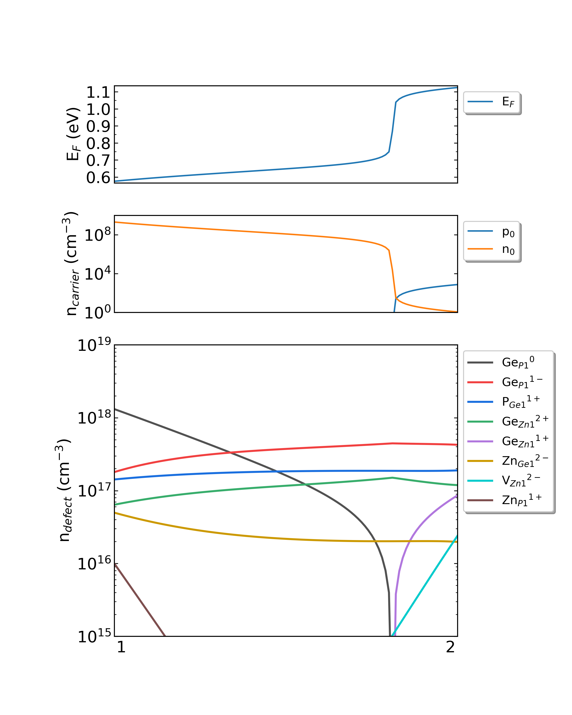
Fig: The Fermi level, electron and hole carrier densities, and defect densities in ZnGeP2 as functions of the chemical potentials changed between 1 and 2. (the growth temperature is 1300 K, and the working temperature is 300 K.)

Users can adjust the growth and working temperatures in file dasp.in to obtain defect densities in different situations. For example, modify the parameters as follows in file dasp.in and run command dasp 4 again to execute the DDC module that can obtain a new image of defect density:

############## DDC Module ##############
ddc_temperature = 800 300
ddc_mass = 0.36 0.54
ddc_path = 1 2

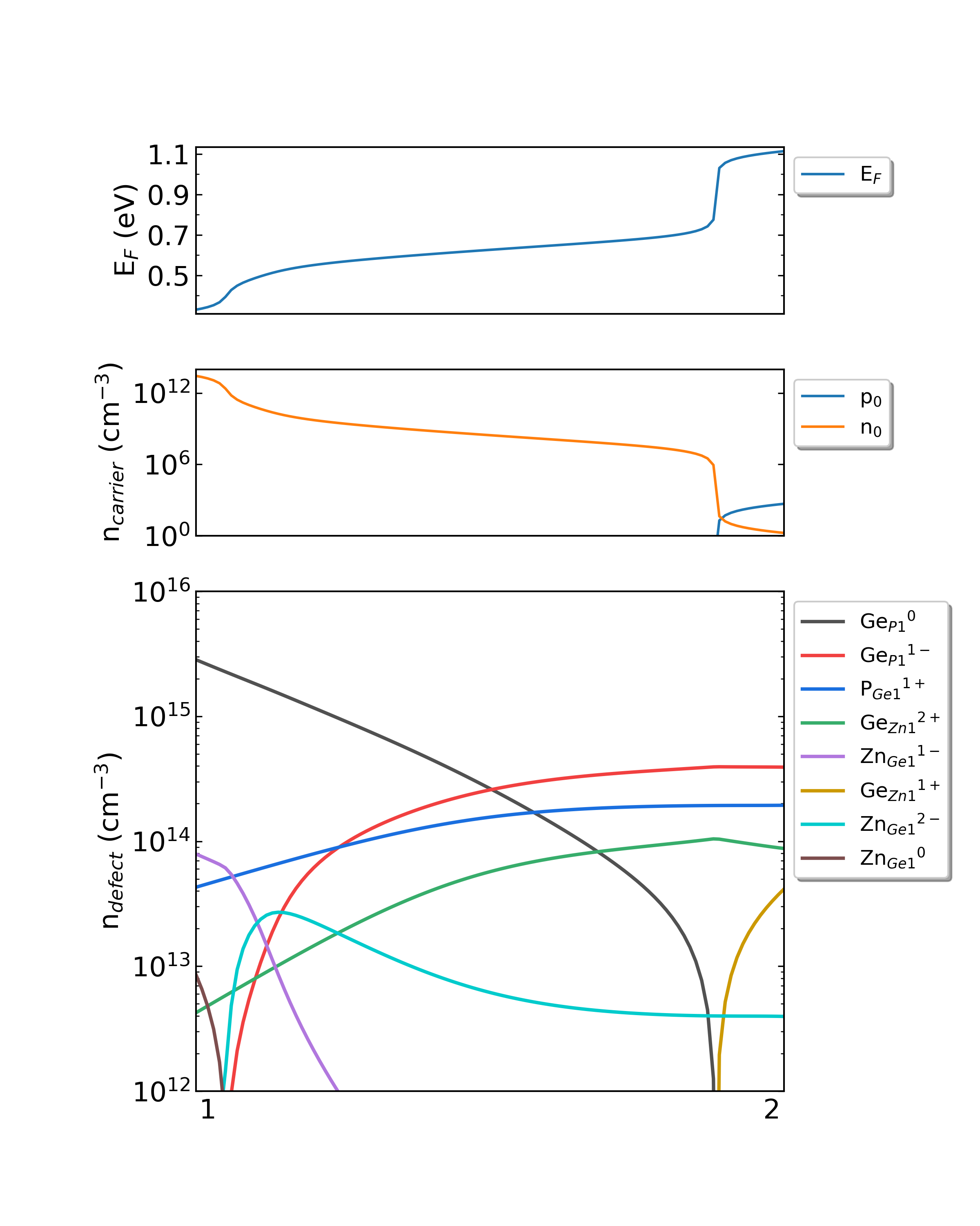
Fig: The Fermi level, electron and hole carrier densities, and defect densities in ZnGeP2 as functions of the chemical potentials changed between 1 and 2. (the growth temperature is 800 K, and the working temperature is 300 K.)

Or

############## DDC Module ##############
ddc_temperature = 300 300
ddc_mass = 0.36 0.54
ddc_path = 1 2

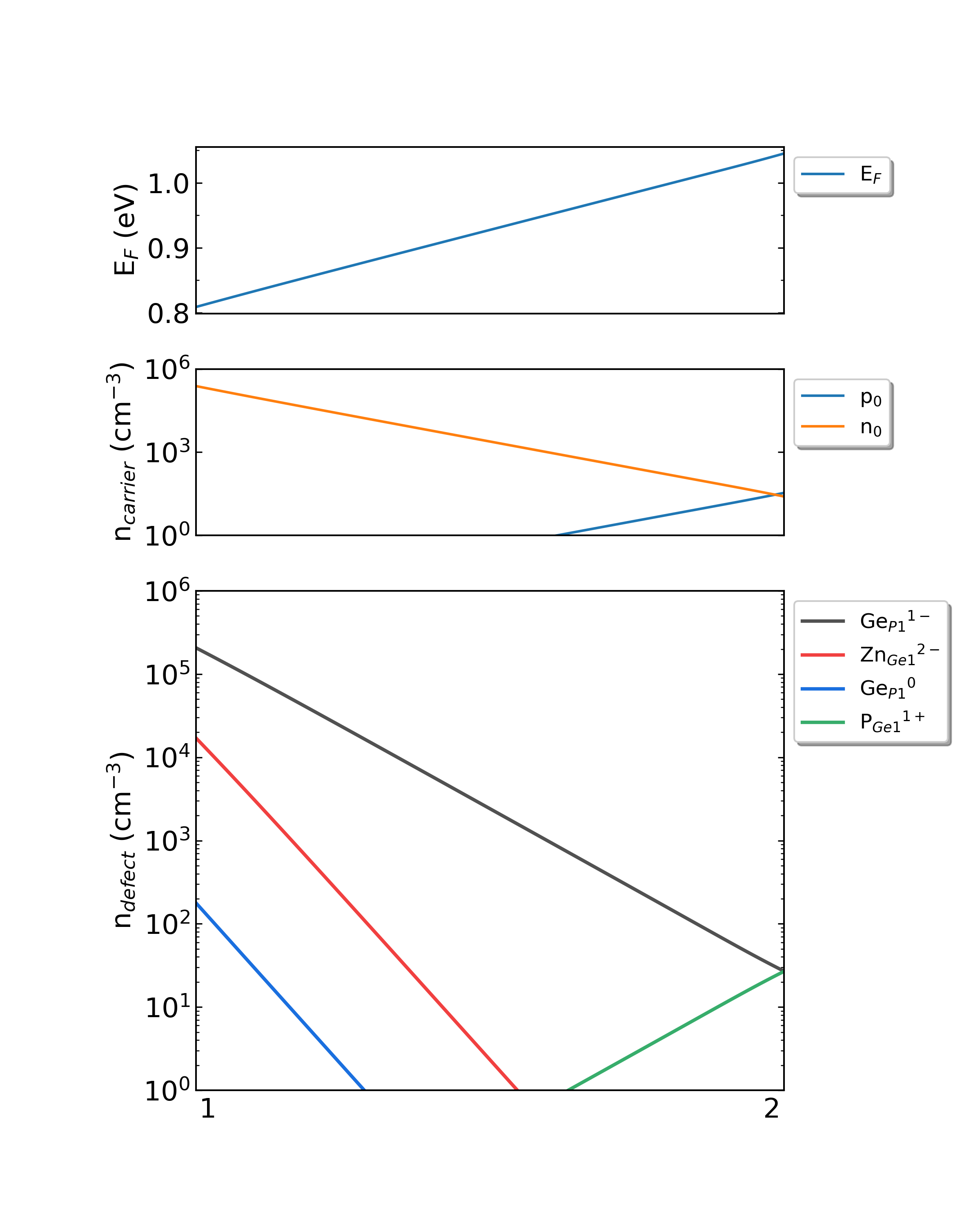
Fig: The Fermi level, electron and hole carrier densities, and defect densities in ZnGeP2 as functions of the chemical potentials changed between 1 and 2. (the growth temperature is 300 K, and the working temperature is 300 K.)

5.4.5 The calculations of radiative transition coefficient and photoluminescence (PL) spectrum¶

5.4.5.1 Run CDC module¶

There have some things that need to be confirmed before using the CDC module:
(1) The DEC module has been completed (the DDC calculation can be skipped).
(2) For the selected defect transition process, the charge states before and after the transition should exist, and the transition energy levels should be in the band gap.
(3) If the radiative capture coefficient needs to be calculated, the VASP source program needs to be modified and recompiled, and the VASP path of the newly compiled version should be filled in vasp_path_cdc in file dasp.in .

For ZnGeP2, we want to calculate the hole trapping process of the defect \(Ge_{Zn}\) from 0 to +1 charge state, so we need to distinguish the band index of the defect level and VBM level in the defect calculation. We recommend that the band index could always be determined by the EIGENVAL file obtained in the static calculation of the neutral defect. For \(Ge_{Zn}\) , the band indexes for VBM and defect level are 864 and 865 respectively, and the process takes place in a spin-down channel judged by EIGENVAL , so the following information can be written into dasp.in :

############## CDC Module ###############
cdc_defect = Ge_Zn1
cdc_job = pl
cdc_charge = 0 1      # The charge state before and after capture is in the front and back respectively.
cdc_band = 864 865     # The band index for band edge and defect level is in the front and back respectively.
cdc_temperature = 300
spin_channel = 2
refractive_index = 2.38

Use comman dasp 5 to execute the CDC module, no additional operation need is required while waiting for the program to complete.

5.4.5.2 Preliminary calculation¶

Firstly, CDC module will judge whether the structural relaxations using HSE functional for the structure of the initial and final state of the selected defect have been completed based on the value of level in dasp.in . If level is 2, CDC module will adopt HSE functional to optimize the structure of the selected defect. If level is 3, CDC module will skip the structure optimization. And if level is 1, CDC module will exit the calculation of this module.

The following comes from the program log file 5cdc.out of CDC module:

----------------------- relaxation calc of initial state -----------------------

finished : /data/home/.../ZnGeP2/cdc/Ge_Zn1/Radiate_calc/_q0_to_q1_/initial_state/relaxation

----------------------- relaxation calc of final state -----------------------

finished : /data/home/.../ZnGeP2/cdc/Ge_Zn1/Radiate_calc/_q0_to_q1_/final_state/relaxation

------------------------------------------------

Next, CDC module will use the structure relaxed by HSE functional to calculate the carrier transition matrix of the initial state and the intermediate state energy of the final state with the initial structure.

The following comes from the program log file 5cdc.out of CDC module:

Ge_Zn1 : from q0 state to q1 state
hole : from 864 band to 865 band

----------------------- static calc of initial state for transition matrix -----------------------

finished : /data/home/.../ZnGeP2/cdc/Ge_Zn1/Radiate_calc/_q0_to_q1_/initial_state/static_optic

----------------------- static calc of intermediate state for relaxation energy -----------------------

finished : /data/home/.../ZnGeP2/cdc/Ge_Zn1/Radiate_calc/_q0_to_q1_/intermediate_state/static

Subsequently, CDC module will calculate the zero-phonon line energy E_zpl based on the transition energy between the two defect states, and the phonon relaxation energy E_rel required by the defect from the initial structure to the final structure based on the energy of the intermediate state and final state, so as to obtain the energy of the radiated photons (E_emission).

The following comes from the program log file 5cdc.out of CDC module:

transition level is 1.4203 eV
E_zpl ( Energy of zero phonon line ) is 1.4203 eV
total energy of the final state with the initial state configuration is -1142.4152 eV
total energy of the final state is -1142.6177 eV
E_rel (the lattice relaxation energy) is 0.2025 eV
E_emission (the emission energy) is 1.2178 eV

5.4.5.3 The flow of radiative capture coefficient calculation¶

After finishing the above calculations, CDC module will calculate the radiative capture coefficient according to the data such as the volume of supercell and carrier effective masses, and the corresponding equation.

The following comes from the program log file 5cdc.out of CDC module:

Radiative carrier capture coefficient is 0.9106*1e-13 cm^3/s

----------------------- End of Calculation for Radiative Capture Rate -----------------------

5.4.5.4 The flow of PL spectrum calculation¶

After obtaining the above data, CDC module will analyze the generalized coordinates difference \(ΔQ\) between the initial and the final state of the defect structure relaxed by HSE functional, and linearly generate a series of structures along this direction.

There will appear many directories for static calculation in the both directories /cdc/Ge_Zn1/Radiate_calc/_q0_to_q1_/final_state and /cdc/Ge_Zn1/Radiate_calc/_q0_to_q1_/initial_state.

Q0  Q10  Q-10  Q2  Q-2  Q4  Q-4  Q6  Q-6  Q8  Q-8

After completing the above calculation, the CDC module can obtain the effective phonon energy, phonon wavefunction, and Huang-Rhys factor of the final state in the initial and final state according to the generated structure and the corresponding defect formation energy, and also obtain the one-dimensional configuration diagram of the initial and final state of the defect. The output is the image ccdiagram.png , as shown in below:

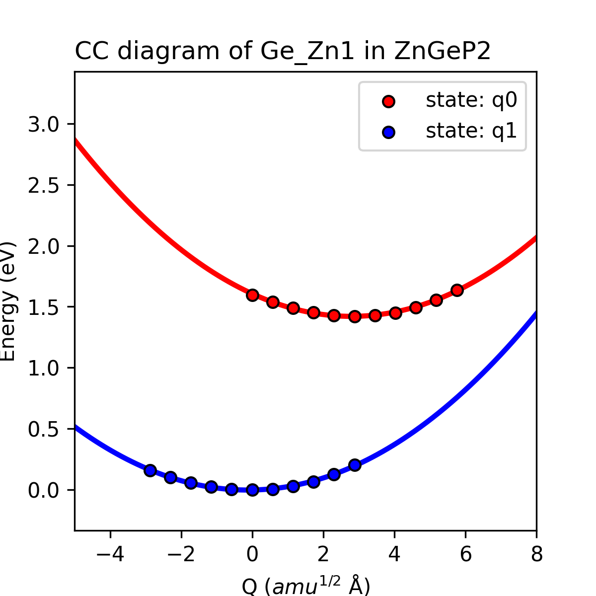
Fig: The one-dimensional configuration diagram of defect Ge_Zn1 in ZnGeP2.

The following comes from the program log file 5cdc.out of CDC module:

----------------------- Calculation for PL Spectrum Start -----------------------

Analysing deltaQ (the structure difference in generalized coordinate) ...
deltaQ between two structures in a.u.:232.2316
deltaQ between two structures in amu^1/2*Angs: 2.879

------------------------------------------------

Generating structures...

...

------------------------------------------------

calculation of initial state and final state all finished

------------------------------------------------

analysing for pl spectrum...

effective phonon energy of the initial state is 0.01397 eV

effective phonon energy of the final state is 0.01338 eV

Huang-Rhys factor of the final state is 15.13453

ccdiagram.png saved in dir /data/home/Zn_Ge_P/cdc/Ge_Zn1/Radiate_calc/_q0_to_q1_

Finally, CDC module will output the raw data file lineshape.dat of the PL spectrum, and also output its peak position and FWHM, at last, save the image in file lineshape.png .

lineshape.dat saved in dir /data/home/cai/daike/Zn_Ge_P/CDC_test_0310/cdc/Ge_Zn1/Radiate_calc/_q0_to_q1_

Position of the peak in the lineshape is 1.26 eV

Full width at half maxima of the lineshape is 0.21 eV

analysis for pl spectrum finished

lineshape.png saved in dir /data/home/Zn_Ge_P//cdc/Ge_Zn1/Radiate_calc/_q0_to_q1_

----------------------- End of Calculation for PL Spectrum -----------------------

The image lineshape.png is shown in below:

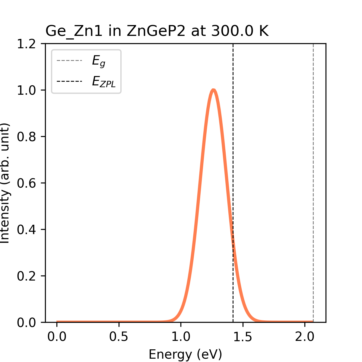
Fig: The PL spectrum of defect Ge_Zn1 in ZnGeP2 at a given temperature.

5.5 Rapid prediction of the stability of double perovskite materials¶

In the above cases, we showed that the TSC module can calculate the element chemical potential and uses it to calculate the formation energy in DEC module. In addition, TSC module can be run independently to analyze the stability of the compound without the need for PREPARE module calculations.

The TSC module can be run directly by setting tsc_only = T in dasp.in . After TSC module finishes the first stage analysis, it will conduct the second stage analysis with level = 1 by itself.

The following examples showed the analysis process of three kinds of double perovskite materials Cs2AgBiCl6, Rb2LiInI, and K2LiYF6.

5.5.1 Cs2AgBiCl6 (Predicted result: stable)¶

5.5.1.1 Prepare files¶

The first step in the material stability analysis using TSC module is still to prepare POSCAR and dasp.in .

The POSCAR of Cs2AgBiCl6 can be obtained from MP database, and the structure needs to be optimized or set by the user. The POSCAR for this case is as follows:

Cs2 Ag1 Bi1 Cl6
00000000000000
7438184481880610    0.0000000000000355    0.0000000000000251
8719092240440918    6.7063434983622878   -0.0000000000000092
8719092240440918    2.2354478328207339    6.3228012862560394
Cs   Ag   Bi   Cl
   1     1     6
Direct
7500000000000000  0.7500000000000000  0.7500000000000000
2500000000000000  0.2500000000000000  0.2500000000000000
5000000000000000  0.5000000000000000  0.5000000000000000
-0.0000000000000000 -0.0000000000000000  0.0000000000000000
7508700137251050  0.2491299562748926  0.2491299562748926
2491299562748926  0.2491299562748926  0.7508700137251050
2491299562748926  0.7508700137251050  0.7508700137251050
2491299562748926  0.7508700137251050  0.2491299562748926
7508700137251050  0.2491299562748926  0.7508700137251050
7508700137251050  0.7508700137251050  0.2491299562748926

Users need to set the relevant parameters in the file dasp.in according to their own situation, and set tsc_only = T and database_api .

############## Job Scheduling ##############
cluster = SLURM     # (job scheduling system)
node_number = 4         # (number of node)
core_per_node = 32      # (core per node)
queue = normal           # (name of queue/partition)
max_time = 24:00:00        # (maximum time for a single DFT calculation)
vasp_path_tsc = /opt/vasp.5.4.4/bin/vasp_std
job_name = submit_job    # (name of script)
potcar_path = /opt/POT/potpaw_PBE    # (path of pseudopotentials)
max_job = 5

############## TSC Module ##############
database_api = ******************* # (str-list type)
tsc_only = T
plot_3d = T

For the parameters of TSC module,

database_api = ******************* # (str-list type)
# use to visit the Materials Project database

tsc_only = T
# Only rapid stability analysis with level = 1 is performed.

plot_3d = T
# For quaternary compounds, TSC module can output three dimensional phase diagram (for user reference only). The default is F, it will be output three dimensional phase diagram by setting to T.

5.5.1.2 Calculation and analysis¶

The total energy calculation of the host structure (the parameters are consistent with MP database):

TSC module will use the same input parameters (INCAR, KPOINTS, POTCAR) with the Materials Project database to perform structural relaxation and static calculation on the primitive cells given by the user. Therefore, the calculated total energy is comparable to that of the MP database. This step is to obtain the key hetero-phases that limit the stability of Cs2AgBiCl6. In the directory, we can see:

cd tsc
cd Cs2AgBiCl6/
ls
relaxation1  relaxation2  static

The running log also can be seen from the Cs2AgBiCl6/tsc/2tsc.out, that is, the steps such as generating input files, relaxation1, relaxation2, static and data extraction.

Rapid analysis of the stability and key hetero-phases compounds:

The TSC module will search for all the secondary compounds that compete with Cs2AgBiCl6 in the MP database. According to the output file materials_info.yaml , it can be found that all the considered hetero-phases compounds including:

secondary_phases:
- - Cs
  - Ag
  - Bi
  - Cl2
  - Ag3Bi
  - Ag2Cl3
  - Ag3Cl
  - AgCl
  - Cs2AgCl3
  - CsAgCl2
  - CsAgCl3
  - Bi6Cl7
  - BiCl3
  - Cs3BiCl6
  - Cs3Bi2Cl9
  - CsBi
  - Cs3Bi2
  - CsBi2
  - Cs3Bi
  - CsCl

By comparing the calculated total energy of Cs2AgBiCl6 with that of the hetero-phases extracted from the database, it can be judged that Cs2AgBiCl6 is thermodynamically stable.

Subsequently, the program will automatically download the key hetero-phases compounds that can limit the thermodynamic stability of Cs2AgBiCl6. Ag, Cs, Bi, Cl2, AgCl, CsAgCl2, Cs3BiCl6, CsAgCl3, and Cl2Cs3Bi2Cl9 are considered in this case. The relevant information can be seen in 2tsc.out :

...
analysing the thermodynamic stability of Cs2AgBiCl6.
The stability of Cs2AgBiCl6 is: True.
key phases of Cs2AgBiCl6 are: AgCl Ag Cs3Bi2Cl9 CsAgCl2 Cs3BiCl6 CsAgCl3 Cs Bi Cl2 .
analysing of Cs2AgBiCl6 is done.
...

Meanwhile, the same information is also output in file materials_info.yaml :

key_phases:
  - AgCl
  - CsAgCl2
  - CsAgCl3
  - Ag
  - Cs3BiCl6
  - Cs3Bi2Cl9
  - Cs
  - Bi
  - Cl2

The total energy calculation of the host and hetero-phase compounds:

As Cs2AgBiCl6 is thermodynamically stable, TSC module will perform the second analysis and calculation after the key hetero-phase compounds are confirmed, i.e. according to the POTCAR files in the path of pseudopotential provided by users, using level=1 to calculate the total energies of Cs2AgBiCl6 and the hetero-phase compounds mentioned above. 2tsc.out is as follows:

...
Job ******** submitted: /home/test/Cs2AgBiCl6/tsc/Cs2AgBiCl6/static_recalc
Job ******** submitted: /home/test/Cs2AgBiCl6/tsc/AgCl/static_recalc
Job ******** submitted: /home/test/Cs2AgBiCl6/tsc/CsAgCl2/static_recalc
...
Succeed job  12267.host2: /home/test/Cs2AgBiCl6/tsc/Cs2AgBiCl6/static_recalc
Succeed job  12269.host2: /home/test/Cs2AgBiCl6/tsc/AgCl/static_recalc
Succeed job  12271.host2: /home/test/Cs2AgBiCl6/tsc/CsAgCl2/static_recalc
...

If there are errors in the calculations, modify the relevant parameters, such as INCAR or KPOINTS , and then run again. The details can be seen in Common problems section.

The chemical potential calculation:

Calculating the formation energy and stable chemical potential region of Cs2AgBiCl6 based on the calculated total energy. TSC module will give the endpoint of eight chemical potentials, and write them into dasp.in :

# The orders are consistent with the order of elements in POSCAR, i.e. the first column is Cs, the second column is Ag, the third column is Bi, and the fourth is Cl.
E_pure = -0.836 -2.6987 -3.8871 -1.7877
p1 = -3.5853 -0.4806 -2.9502 -0.5666
p2 = -3.1047 -0.0 -1.5084 -1.0472
p3 = -4.1861 -0.781 -3.2506 -0.2662
p4 = -3.4051 -0.0 -0.9076 -1.0472
p5 = -3.5373 -0.5286 -2.9982 -0.5666
p6 = -3.0087 0.0 -1.4124 -1.0952
p7 = -3.7897 -0.781 -3.2506 -0.3983
p8 = -3.0087 -0.0 -0.9076 -1.1793

The output after the program is completed can be seen in 2tsc.out :

analysing the thermodynamic stability of Cs2AgBiCl6.
The stability of Cs2AgBiCl6 is: True.
key phases of Cs2AgBiCl6 are: AgCl Ag Cs3Bi2Cl9 CsAgCl2 Cs3BiCl6 CsAgCl3 Cs Bi Cl2 .
analysing of Cs2AgBiCl6 is done.
sub-module of tsc: 'auto thermodynamic calculation' ends successfully.
---------------------------
DASP-TSC finished

For the ternary and multinary compounds, TSC module will output the image of the stable region and the chemical potential at the endpoint of the stable region. For the two dimensional figures, it can be seen through this directory:

cd tsc
cd 2d-figures/
ls
fig-Cs2AgBiCl6.png  fig-Cs2AgBiCl6_recalc.png  stable_2d.out stable_recalc_2d.out

The four files under the directory Cs2AgBiCl6/tsc/2d-figures/ are the images of the stable region plotted during the two calculations and analyses, and the chemical potential at each endpoint in the images.

Check out the files stable_2d.out and fig-Cs2AgBiCl6.png . The horizontal and vertical coordinates of fig-Cs2AgBiCl6.png are the chemical potential of the elements marked in the figure, and the shaded area is the stable region of the host compound. Each line on the boundary is the chemical potential curve at the critical condition where the marked material can or can not form. This is the image output from the first calculation and analysis process.

     Bi       Ag       Cs       Cl
-------  -------  -------  -------
-2.9709  -0.3807  -3.5994  -0.5224
-3.1086  -0.5184  -3.5994  -0.4765
-2.8656  -0.5184  -3.5994  -0.517
-1.6748  -0.1214  -3.5994  -0.7817

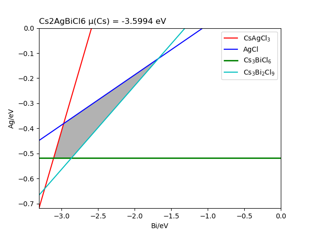
Fig: The stable chemical potential region of Cs2AgBiCl6. (comes from the MP database)

Check out the files stable_recalc_2d.out and fig-Cs2AgBiCl6_recalc.png . They are the image and data output from the second calculation and analysis process.

     Bi       Ag       Cs       Cl
-------  -------  -------  -------
-2.9562  -0.4866  -3.5974  -0.5606
-3.0583  -0.5887  -3.5974  -0.5265
-2.6737  -0.5887  -3.5974  -0.5906
-1.4845  -0.1923  -3.5974  -0.8549

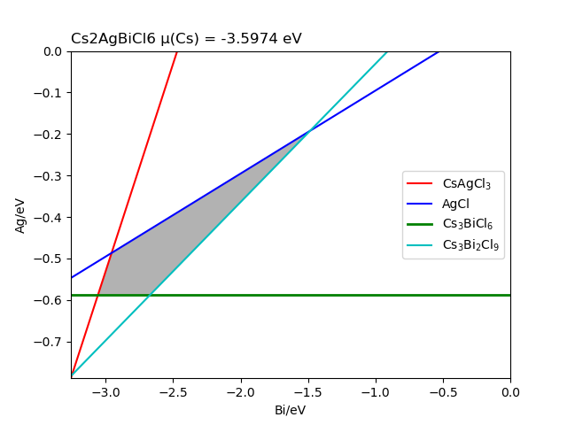
Fig: The stable chemical potential region of Cs2AgBiCl6. (comes from the second stage calculations)

For the three dimensional figures, it can be seen through this directory:

cd tsc
cd 3d-figures/
ls
fig-Cs2AgBiCl6_3d.png  fig-Cs2AgBiCl6_3d_recalc.png  stable.out  stable_recalc.out

The four files under the directory Cs2AgBiCl6/tsc/3d-figures/ are the images of the stable region plotted during the two calculations and analyses, and the chemical potential at each endpoint in the images.

Check out the files stable.out and fig-Cs2AgBiCl6_3d.png . The chemical potentials of the three elements marked in fig-Cs2AgBiCl6_3d.png constitute three coordinate axes, and the area surrounded by red lines is the three-dimensional stable region of Cs2AgBiCl6. This is the image output from the first calculation and analysis process, and the coordinates of each point in this region can be obtained from the file stable.out .

     Cs            Ag        Bi         Cl
--------  ------------  --------  ---------
-3.17837   6.73289e-17  -1.90967  -0.903106
-3.47796  -0            -1.31049  -0.903106
-3.08102  -3.47289e-18  -1.81231  -0.951782
-3.08102  -0            -1.31049  -1.03542
-3.51867  -0.340294     -2.93055  -0.562812
-4.11785  -0.639883     -3.23014  -0.263223
-3.46999  -0.38897      -2.97922  -0.562812
-3.7209   -0.639883     -3.23014  -0.395537

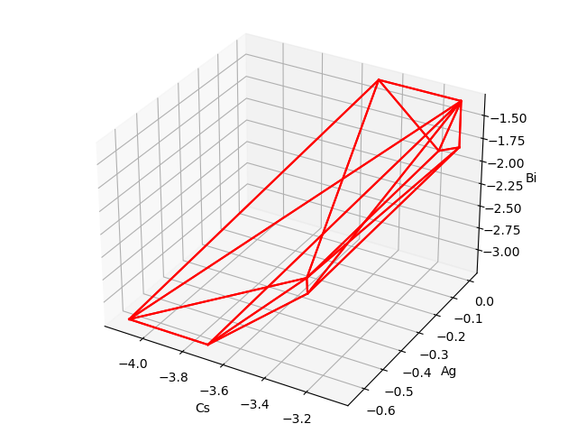
Fig: The 3D stable chemical potential region of Cs2AgBiCl6. (comes from the MP database)

Check out the files stable_recalc_3d.out and fig-Cs2AgBiCl6_3d_recalc.png . They are the image and data output from the second calculation and analysis process.

     Cs            Ag       Bi         Cl
-------  ------------  -------  ---------
-3.5853  -0.4806       -2.9502  -0.5666
-3.1047  -3.63857e-17  -1.5084  -1.0472
-4.1861  -0.781        -3.2506  -0.2662
-3.4051  -0            -0.9076  -1.0472
-3.5373  -0.5286       -2.9982  -0.5666
-3.0087   0            -1.4124  -1.0952
-3.7897  -0.781        -3.2506  -0.398333
-3.0087  -0            -0.9076  -1.17933

Fig: The 3D stable chemical potential region of Cs2AgBiCl6. (comes from the second stage calculations)

5.5.2 K2LiYF6 (Predicted result: unstable)¶

5.5.2.1 Prepare POSCAR and dasp.in¶

The POSCAR of K2LiYF6 can be obtained from MP database, and the structure needs to be optimized or set by the user. The POSCAR for this case is as follows:

K8 Li4 Y4 F24
0
557390 0.000000 0.000000
000000 8.557390 0.000000
000000 0.000000 8.557390
K Li Y F
4 4 24
direct
250000 0.250000 0.750000 K
250000 0.750000 0.750000 K
250000 0.750000 0.250000 K
250000 0.250000 0.250000 K
750000 0.250000 0.250000 K
750000 0.750000 0.250000 K
750000 0.750000 0.750000 K
750000 0.250000 0.750000 K
500000 0.000000 0.000000 Li
500000 0.500000 0.500000 Li
000000 0.000000 0.500000 Li
000000 0.500000 0.000000 Li
...

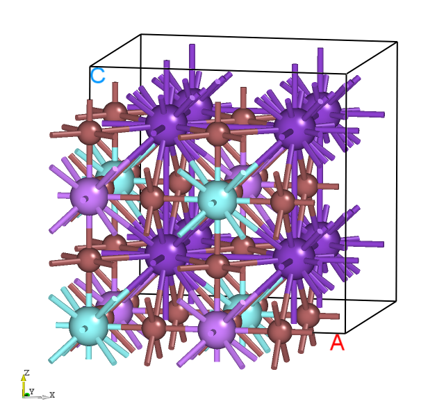
Fig: The crystal structure schematic of K2LiYF6.

Users need to set the relevant parameters in the file dasp.in according to their own situation, and set tsc_only = T and database_api . The details can refer to Cs2AgBiCl6.

5.5.2.2 Calculation and analysis¶

The total energy calculation of the host structure (the parameters are consistent with MP database):

TSC module will use the same input parameters (INCAR, KPOINTS, POTCAR) with the Materials Project database to perform structural relaxation and static calculation on the primitive cells given by the user. Therefore, the calculated total energy is comparable to that of the MP database. This step is to obtain the key hetero-phases that limit the stability of K2LiYF6. In the directory, we can see:

cd tsc
cd K2LiYF6/
ls
relaxation1  relaxation2  static

The running log also can be seen from the K2LiYF6/tsc/2tsc.out, that is, the steps such as generating input files, relaxation1, relaxation2, static and data extraction.

Rapid analysis of the stability and key hetero-phases compounds:

The TSC module will search for all the secondary compounds that compete with K2LiYF6 in the MP database. According to the output file materials_info.yaml , it can be found that all the considered hetero-phases compounds including:

secondary_phases:
- - K
  - Li
  - Y
  - F
  - KF2
  - KF3
  - KF
  - KF5
  - KLiYF5
  - K3YF6
  - KYF4
  - K2YF5
  - KY3F10
  - KY2F7
  - LiF
  - LiF3
  - LiYF4
  - LiYF2
  - Li3YF6
  - YF3
  - K3Li
  - KLi3
  - K3Y
  - LiY3
  - Li3Y

By comparing the calculated total energy of Cs2AgBiCl6 with that of the hetero-phases extracted from the database, it can be judged that Cs2AgBiCl6 is unstable. The relevant information can be seen in 2tsc.out :

...
analysing the thermodynamic stability of K2LiYF6.
The stability of K2LiYF6 is: False.
K2LiYF6 may decompose into ['K2YF5', 'K2YF5'].
you can set tag: 'excluded_phase' to get some reference values of chemical potentials.
analysing of K2LiYF6 is done.
...

The value of energy above hull of K2LiYF6 is output in file materials_info.yaml , it is positive and consistent with the result that “this compound is unstable”.

e_above_hull: 0.0466

The decomposed products include K2YF5 and LiF, and this also can be known from the output file materials_info.yaml :

decomp:
- K2YF5
- LiF

As K2LiYF6 is unstable, TSC module can not judge the key hetero-phase compounds or output the images of the stable region. Moreover, TSC module will not do the calculation of the second stage further.

If users still want to do the second stage calculations to obtain the stable chemical potential region, they can set excluded_phase to exclude the effect of some hetero-phase compounds on the stability of the host compound based on the prompt in file 2tsc.out . Generally, one or more of the decompositions is excluded to make the host compound has a referable stable region. i.e. set excluded_phase = LiF , or excluded_phase = K2YF5 , or excluded_phase = LiF K2YF5 in file dasp.in , and run TSC module again. At this point, it is possible that the compound is still unstable, then some compounds in the current decomposition path can be appended to excluded_phase and re-run the TSC module.

5.5.2.3 Additional calculation and analysis¶

In this case, the parameters in file dasp.in that may make the host compound has a stable region after excluding some certain hetero-phase compounds are as follows:

############## Job Scheduling ##############
cluster = SLURM     # (job scheduling system)
node_number = 4         # (number of node)
core_per_node = 32      # (core per node)
queue = normal           # (name of queue/partition)
max_time = 24:00:00        # (maximum time for a single DFT calculation)
vasp_path_tsc = /opt/vasp.5.4.4/bin/vasp_std
job_name = submit_job    # (name of script)
potcar_path = /opt/POT/potpaw_PBE    # (path of pseudopotentials)
max_job = 5

############## TSC Module ##############
database_api = ******************* # (str-list type)
tsc_only = T
plot_3d = T
excluded_phase = K2LiYF6 K2YF5 LiF KLiYF5 LiYF4

The excluded phases include K2LiYF6, K2YF5, LiF, KLiYF5, and LiYF4.

For the unstable compounds, the stable region may be different because the hetero-phases excluded are different, the above parameters are for reference only.

As the total energy calculations have already been done, so the relevant stability analysis information can be seen in file 2tsc.out quickly:

analysing the thermodynamic stability of K2LiYF6.
excluded phase of K2LiYF6: K2LiYF6 K2YF5 LiF KLiYF5 LiYF4 .
The stability of K2LiYF6 is: True.
key phases of K2LiYF6 are: KYF4 K3YF6 Li3YF6 KF2 KF Li KY3F10 KY2F7 F2 K Y .
file key_phases_info_recalc.yaml generated.
analysing of K2LiYF6 is done.

And the second stage calculations have begun for the key hetero-phase compounds mentioned above, shown in 2tsc.out as below:

...
Job ******** submitted: /home/fudan/daike/KLiYF/DASP_0219/tsc/K2LiYF6/static_recalc
Job ******** submitted: /home/fudan/daike/KLiYF/DASP_0219/tsc/KYF4/static_recalc
Job ******** submitted: /home/fudan/daike/KLiYF/DASP_0219/tsc/K3YF6/static_recalc
Job ******** submitted: /home/fudan/daike/KLiYF/DASP_0219/tsc/Li3YF6/static_recalc
...
Succeed job  ********: /home/fudan/daike/KLiYF/DASP_0219/tsc/K2LiYF6/static_recalc
Succeed job  ********: /home/fudan/daike/KLiYF/DASP_0219/tsc/KYF4/static_recalc
Succeed job  ********: /home/fudan/daike/KLiYF/DASP_0219/tsc/K3YF6/static_recalc
Succeed job  ********: /home/fudan/daike/KLiYF/DASP_0219/tsc/KF2/static_recalc

...

If there are errors in the calculations, modify the relevant parameters, such as INCAR or KPOINTS , and then run again. The details can be seen in Common problems section.

The chemical potential calculation:

Calculating the formation energy and stable chemical potential region of K2LiYF6 based on the calculated total energy. TSC module will give the endpoint of 14 chemical potentials, and write them into dasp.in :

# The orders are consistent with the order of elements in POSCAR, i.e. the first column is K, the second column is Li, the third column is Y, and the fourth is F.
E_pure = -1.086 -1.8579 -6.453 -1.8583
p1 = -0.0059 0.0 -0.1727 -5.5633
p2 = -5.5692 -5.5633 -16.8626 0.0
p3 = -0.4569 0.0 -0.6237 -5.3378
p4 = -5.7947 -5.3378 -16.6371 0.0
p5 = -5.4204 -5.4145 -16.9064 -0.0671
p6 = -5.5546 -5.5487 -16.9064 0.0
p7 = -0.0059 0.0 -0.6629 -5.4816
p8 = -5.4204 -4.1335 -18.1874 -0.0671
p9 = -5.5546 -4.2677 -18.1874 0.0
p10 = -1.2869 0.0 -5.7869 -4.2006
p11 = -1.2869 0.0 -2.0624 -4.8213
p12 = -6.1083 -4.8213 -16.5265 0.0
p13 = -0.5489 0.0 -0.7709 -5.2826
p14 = -5.8315 -5.2826 -16.6187 0.0

The output after the program is completed can be seen in 2tsc.out :

analysing the thermodynamic stability of K2LiYF6.
excluded phase of K2LiYF6: K2LiYF6 K2YF5 LiF KLiYF5 LiYF4 .
The stability of K2LiYF6 is: True.
key phases of K2LiYF6 are: K3YF6 Li3YF6 KF2 KF KYF4 F2 Li KY3F10 KY2F7 K Y .
analysing of K2LiYF6 is done.
sub-module of tsc: 'auto thermodynamic calculation' ends successfully.
---------------------------
DASP-TSC finished

For the ternary and multinary compounds, TSC module will output the image of the stable region and the chemical potential at the endpoint of the stable region. For the two dimensional figures, it can be seen through this directory:

cd tsc
cd 2d-figures/
ls
fig-K2LiYF6.png  fig-K2LiYF6_recalc.png  stable_2d.out stable_recalc_2d.out

The four files under the directory K2LiYF6/tsc/2d-figures/ are the images of the stable region plotted during the two calculations and analyses, and the chemical potential at each endpoint in the images.

Check out the files stable_2d.out and fig-K2LiYF6.png . The horizontal and vertical coordinates of fig-K2LiYF6.png are the chemical potential of the elements marked in the figure, and the shaded area is the stable region of the host compound. Each line on the boundary is the chemical potential curve at the critical condition where the marked material can or can not form. This is the image output from the first calculation and analysis process.

       Y       Li        K        F
--------  -------  -------  -------
-7.3952  -1.7304  -3.0425  -3.0094
-11.1139  -1.7304  -3.0425  -2.3896
-9.8349  -3.0094  -3.0425  -2.3896
-9.3452  -3.0094  -3.0425  -2.4712
-8.4446  -2.5591  -3.0425  -2.6964
-8.3183  -2.4689  -3.0425  -2.7325

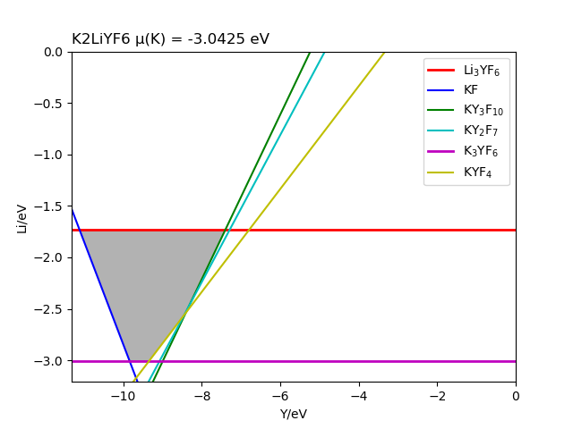
Fig: The stable chemical potential region of K2LiYF6. (comes from the MP database)

Check out the files stable_recalc_2d.out and fig-K2LiYF6_recalc.png . They are the image and data output from the second calculation and analysis process.

     Y       Li        K        F
--------  -------  -------  -------
-7.373   -1.7702  -3.0571  -3.0512
-11.0975  -1.7702  -3.0571  -2.4304
-9.8165  -3.0512  -3.0571  -2.4304
-9.3263  -3.0512  -3.0571  -2.5121
-8.4243  -2.6002  -3.0571  -2.7376
-8.2955  -2.5082  -3.0571  -2.7744

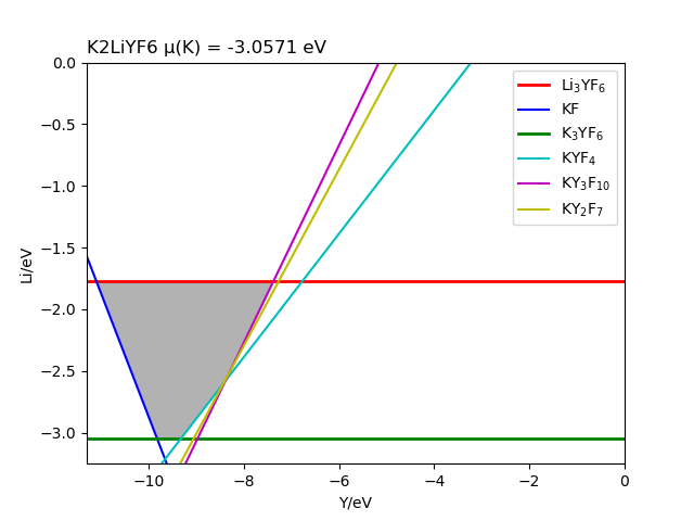
Fig: The stable chemical potential region of K2LiYF6. (comes from the second stage calculations)

For the three dimensional figures, it can be seen through this directory:

cd tsc
cd 3d-figures/
ls
fig-K2LiYF6_3d.png  fig-K2LiYF6_3d_recalc.png  stable.out  stable_recalc.out

The four files under the directory K2LiYF6/tsc/3d-figures/ are the images of the stable region plotted during the two calculations and analyses, and the chemical potential at each endpoint in the images.

Check out the files stable.out and fig-K2LiYF6_3d.png . The chemical potentials of the three elements marked in fig-K2LiYF6_3d.png constitute three coordinate axes, and the area surrounded by red lines is the three-dimensional stable region of K2LiYF6. This is the image output from the first calculation and analysis process, and the coordinates of each point in this region can be obtained from the file stable.out .

     K            Li           Y             F
----------  ------------  ----------  ------------
-0.0331078   0             -0.806716  -5.39901
-1.31209     0             -5.92265   -4.12003
-0.0331078   0             -0.316988  -5.48063
-0.483403    0             -0.767283  -5.25549
-0.573574    0             -0.911557  -5.20138
-1.31209     2.75724e-17   -2.20396   -4.73981
-5.49866    -5.46555      -16.8041     5.92119e-16
-5.49866    -4.18657      -18.0831     5.92119e-16
-5.51374    -5.48063      -16.7589     1.77636e-15
-5.73889    -5.25549      -16.5337     1.77636e-15
-5.77496    -5.20138      -16.5157     1.18424e-15
-6.0519     -4.73981      -16.4234     0
-5.36558    -5.33247      -16.8041    -0.0665391
-5.36558    -4.05349      -18.0831    -0.0665391

Fig: The 3D stable chemical potential region of K2LiYF6. (comes from the MP database)

Check out the files stable_recalc_3d.out and fig-K2LiYF6_3d_recalc.png . They are the image and data output from the second calculation and analysis process.

     K            Li         Y             F
--------  ------------  --------  ------------
-0.0059    0             -0.1727  -5.5633
-5.5692   -5.5633       -16.8626   0
-0.4569    0             -0.6237  -5.3378
-5.7947   -5.3378       -16.6371   0
-5.4204   -5.4145       -16.9064  -0.0671
-5.5546   -5.5487       -16.9064   0
-0.0059    0             -0.6629  -5.4816
-5.4204   -4.1335       -18.1874  -0.0671
-5.5546   -4.2677       -18.1874   5.92119e-16
-1.2869    0             -5.7869  -4.2006
-1.2869    1.56171e-17   -2.0624  -4.82135
-6.10825  -4.82135      -16.5265   0
-0.5489    0             -0.7709  -5.2826
-5.8315   -5.2826       -16.6187   5.92119e-16

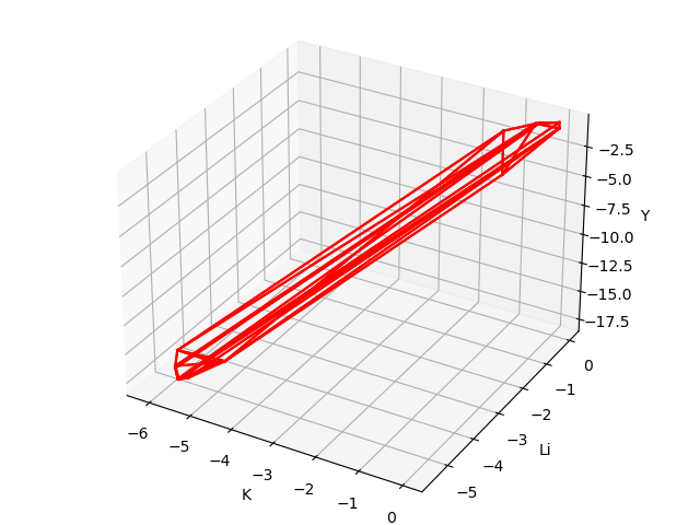
Fig: The 3D stable chemical potential region of K2LiYF6. (comes from the second stage calculations)

5.5.3 Rb2LiInI6 (Predicted result: unstable)¶

5.5.3.1 Prepare POSCAR and dasp.in¶

The POSCAR of Rb2LiInI6 can be obtained from MP database, and the structure needs to be optimized or set by the user. The POSCAR for this case is as follows:

Rb2 Li1 In1 I6
1.0
        7.7485766411         0.0000000000         0.0000000000
        3.8742883205         6.7104642143         0.0000000000
        3.8742883205         2.2368214048         6.3266863345
Rb   Li   In   I
2    1    1    6
Direct
0.750000000         0.750000000         0.750000000
0.250000000         0.250000000         0.250000000
0.500000000         0.500000000         0.500000000
0.000000000         0.000000000         0.000000000
0.750886977         0.249112993         0.249112993
0.249112993         0.249112993         0.750886977
0.249112993         0.750886977         0.750886977
0.249112993         0.750886977         0.249112993
0.750886977         0.249112993         0.750886977
0.750886977         0.750886977         0.249112993

Users need to set the relevant parameters in the file dasp.in according to their own situation, and set tsc_only = T and database_api . The details can refer to Cs2AgBiCl6.

5.5.3.2 Calculation and analysis¶

The total energy calculation of the host structure (the parameters are consistent with MP database):

TSC module will use the same input parameters (INCAR, KPOINTS, POTCAR) with the Materials Project database to perform structural relaxation and static calculation on the primitive cells given by the user. Therefore, the calculated total energy is comparable to that of the MP database. (refer to the previous cases)

Rapid analysis of the stability and key hetero-phases compounds:

The TSC module will search for all the secondary compounds that compete with Rb2LiInI6 in the MP database. According to the output file materials_info.yaml , it can be found that all the considered hetero-phases compounds including:

secondary_phases:
- - Rb
  - Li
  - In
  - I
  - InI4
  - InI3
  - InI
  - InI2
  - LiInI4
  - Rb3InI6
  - RbInI3
  - RbInI4
  - LiI
  - RbI
  - RbI3
  - LiIn3
  - Li3In
  - LiIn
  - LiIn2
  - Li5In4
  - Li2In
  - Li13In3
  - Li3In2
  - Rb3In
  - RbIn4
  - Rb2In3
  - Rb8In11
  - Rb3Li

By comparing the calculated total energy of Rb2LiInI6 with that of the hetero-phases extracted from the database, it can be judged that Rb2LiInI6 is unstable. The relevant information can be seen in 2tsc.out :

...
analysing the thermodynamic stability of Rb2LiInI6.
The stability of Rb2LiInI6 is: False.
Rb2LiInI6 may decomposed into ['RbInI4', 'LiI', 'RbI'].
you can set tag: 'excluded_phase' to get some reference values of chemical potentials.
analysing of Rb2LiInI6 is done.
...

The value of energy above hull of Rb2LiInI6 is output in file materials_info.yaml, it is positive and consistent with the result that “this compound is unstable”.

e_above_hull: 0.0819

The decomposed products include RbInI4, LiI, and RbI, and this also can be known from the output file materials_info.yaml :

decomp:
- RbInI4
- LiI
- RbI

As Rb2LiInI6 is unstable, TSC module can not judge the key hetero-phase compounds or output the images of the stable region. Moreover, TSC module will not do the calculation of the second stage further.

If users still want to do the second stage calculations to obtain the stable chemical potential region, they can set excluded_phase to exclude the effect of some hetero-phase compounds on the stability of the host compound based on the prompt in file 2tsc.out . Generally, one or more of the decompositions is excluded to make the host compound has a referable stable region.

i.e. set excluded_phase = RbInI4 , or excluded_phase = LiI , or excluded_phase = RbInI4 RbI in file dasp.in , and run TSC module again. At this point, it is possible that the compound is still unstable, then some compounds in the current decomposition path can be appended to excluded_phase and re-run the TSC module. (refer to the analysis process of K2LiYF6.)