8 Auxiliary Tool User Guide
备注
Want to quickly analyze results, plot data, or perform common data processing tasks after completing a DFT calculation with DSPAW?
dspawpy (Python >= 3.9) is such a tool. It can be called programmatically (see example scripts below) and also provides a command-line interactive program.
After following the tutorial installation instructions, you can use the interactive program by typing dspawpy and pressing Enter in the command line:
 ... loading dspawpy cli ...

 This is the dspawpy command-line interactive tool.  Enjoy!
    ( )
   _| |  ___  _ _      _ _  _   _   _  _ _    _   _
 /'_` |/',__)( '_`\  /'_` )( ) ( ) ( )( '_`\ ( ) ( )
( (_| |\__, \| (_) )( (_| || \_/ \_/ || (_) )| (_) |
 \__,_)(____/| ,__/'`\__,_) \___x___/ | ,__/  \__, |
             | |                      | |    ( )_| |
             (_)                      (_)     \___/

 Version: Installation Path

 ======================================
 |  1: Update
 |  2: structure conversion
 |  3: Volumetric data processing
 |  4: Band structure calculation
 |  5: Density of States (DOS) data processing
 |  6: Joint display of band structure and density of states (DOS)
 |  7: Optical properties data processing
 |  8: NEB (Nudged Elastic Band) transition state calculation data processing
 |  9: phonon calculation data processing
 |  10: aimd ab initio molecular dynamics data processing
 |  11: Polarization data processing
 |  12: ZPE zero-point energy data processing
 |  13: Thermal correction energy of TS
 |
 |  q: Quit
 ======================================
 --> Enter a number and press Enter to select a function:
Highlights:
Autocompletion: Works by pressing the Tab key, helping to quickly and correctly enter the required program arguments.
Multithreaded lazy loading: Loads modules in the background while waiting for user input, significantly reducing waiting time; loads only necessary modules, minimizing memory usage.
Note:
When using on a remote server, the startup time may be longer due to poor disk I/O performance, potentially taking up to half a minute in extreme cases (directly related to the server’s current disk I/O performance). If this is unacceptable, please install and use dspawpy on your own computer.
After typing dspawpy and pressing Enter, Python will first load built-in modules. Once this is complete, the prompt “… loading dspawpy cli …” will appear, indicating the second stage (loading third-party dependencies) has begun.
After the second stage is completed, a welcome screen will be displayed, indicating that dspwapy has finished the initial loading and has entered the third stage. Subsequently, it will dynamically load the corresponding dependency libraries based on the selected functional modules, thereby minimizing waiting time.
8.1 Installation and Updates
On the HZW machine, dspawpy has been pre-installed. Activate the virtual environment using the following command to start using it:
source /data/hzwtech/profile/dspawpy.env
On other machines, please install dspawpy yourself (choose one of the following two methods):
Using mamba or conda, you can install the package from https://conda-forge.org/download/.
mamba install dspawpy -c conda-forge
#conda install dspawpy -c conda-forge
Or, use pip3 (some operating systems may not have the executable pip3, in which case try pip)
pip
pip3 is the package manager that comes with python3.
Linux and Mac usually come with Python 3 and pip3.
On Windows, open the Microsoft Store, search for Python, and install it.
Then open cmd or powershell to use pip.
pip3 install dspawpy
For information on how to configure pip and conda mirror addresses to speed up the installation process, please refer to https://mirrors.tuna.tsinghua.edu.cn/help/pypi/ and https://mirrors.tuna.tsinghua.edu.cn/help/anaconda/.
If the installation still fails, try the mamba/conda installation method above.
警告
On clusters, due to permission issues, the pip in the public path may not support global installation of Python libraries. You must add the –user option after pip install to install them in your home directory under ~/.local/lib/python3.x/site-packages/, where 3.x represents the Python interpreter version, and x can be any integer between 9 and 13.
Python will prioritize loading dspawpy from the home directory, even if the version in the public environment is newer!
Therefore, if you have previously installed dspawpy with --user and have forgotten to manually update the old version in your home directory, even after sourcing the public environment, you will not be able to call the dspawpy in the public environment. Instead, the old version will still be used, leading to some bugs.
Therefore, considering that the HZW cluster automatically updates dspawpy weekly, it is recommended not to install it redundantly in your home directory; delete any existing installations. On other clusters, ensure that you manually update dspawpy in your home directory in a timely manner.
If you prefer not to delete and update the dspawpy in your home directory, you can use the -s option when running your Python scripts to prevent importing dspawpy from your home directory: python -s your-script.py.
Update dspawpy
To update dspawpy if it was installed with mamba/conda, use the following command:
mamba update dspawpy
#conda update dspawpy
If dspawpy was installed via pip:
pip install dspawpy -U # -U for upgrading to the latest version
备注
If pip uses a domestic mirror site, it may fail to upgrade smoothly because the mirror site has not yet synchronized the latest version of dspawpy ![]() . Please use the following command to tell pip to download and install from the official PyPI site:
. Please use the following command to tell pip to download and install from the official PyPI site:
pip install dspawpy -i https://pypi.org/simple --user -U # -i specifies the download address, --user installs for the current user only, and -U installs the latest version
If you encounter errors related to dspawpy during runtime, first verify that you have correctly imported the latest version of dspawpy and check the installation path:
$ python3 # or python

>>> import dspawpy
>>> dspawpy.__version__ # will output the version number
>>> dspawpy.__file__ # will output the installation path
8.2 structure structure conversion
To read structure information, use the read function; to write structure information to a file, use the write function; for quick structure conversion, use the convert function:
See the 2conversion.py script for conversion:
 1# coding:utf-8
 2from dspawpy.io.structure import convert
 3
 4convert(
 5    infile="dspawpy_proj/dspawpy_tests/inputs/2.1/relax.h5",  # Structure to be converted, if in the current path, you can just write the filename
 6    si=None,  # Select configuration number, if not specified, read all by default
 7    ele=None,  # Filter element symbol, default reads atomic information for all elements
 8    ai=None,  # Filter atomic indices, starting from 1, default to read all atomic information
 9    infmt=None,  # Input structure file type, e.g., 'h5'. If None, it will be matched ambiguously based on the filename rule.
10    task="relax",  # Task type, this parameter is only valid when infile is a folder rather than a filename
11    outfile="dspawpy_proj/dspawpy_tests/outputs/us/relaxed.xyz",  # Structure file name
12    outfmt=None,  # Output structure file type, e.g., 'xyz'. If None, it will be fuzzy matched according to filename rules.
13    coords_are_cartesian=True,  # Written in Cartesian coordinates by default
14)
The rules for setting several key parameters of the convert function are shown in the table below:
infmt (input file format) |
infile (Input file name fuzzy match) |
outfmt (output file format) |
outfile (output filename fuzzy match) |
Description |
|---|---|---|---|---|
h5 |
*.h5 |
X |
X |
HDF5 files saved after DS-PAW calculations are completed |
json |
*.json |
json |
*.json |
json files saved after DS-PAW calculations are completed |
pdb |
*.pdb |
pdb |
*.pdb |
Protein Data Bank |
as |
*.as |
as |
*.as |
DS-PAW structure file containing atomic coordinates and other information |
hzw |
*.hzw |
hzw |
*.hzw |
DeviceStudio’s default structure file |
xyz |
*.xyz |
xyz |
*.xyz |
Supports only single conformation of molecular structure when reading, and extended-xyz type trajectory files including unit cell when writing |
X |
X |
dump |
*.dump |
LAMMPS dump-type trajectory files |
X |
*.cif*/*.mcif* |
cif/mcif |
*.cif*/*.mcif* |
Crystallographic Information File |
X |
*POSCAR*/*CONTCAR*/*.vasp/CHGCAR*/LOCPOT*/vasprun*.xml* |
poscar |
*POSCAR* |
VASP files |
X |
*.cssr* |
cssr |
*.cssr* |
Crystal Structure Standard Representation |
X |
*.yaml/*.yml |
yaml/yml |
*.yaml/*.yml |
YAML Ain’t Markup Language |
X |
*.xsf* |
xsf |
*.xsf* |
eXtended Structural Format |
X |
*rndstr.in*/*lat.in*/*bestsqs* |
mcsqs |
*rndstr.in*/*lat.in*/*bestsqs* |
Monte Carlo Special Quasirandom Structure |
X |
inp*.xml/*.in*/inp_* |
fleur-inpgen |
*.in* |
FLEUR structure file, requires the additional installation of the pymatgen-io-fleur library |
X |
*.res |
res |
*.res |
ShelX res structure file |
X |
*.config*/*.pwmat* |
pwmat |
*.config/*.pwmat |
PWmat files |
X |
X |
prismatic |
*prismatic* |
A file format used for STEM simulations |
X |
CTRL* |
X |
X |
Stuttgart LMTO-ASA files |
备注
In the table above, * represents any character, and X indicates unsupported formats.
h5, json, pdb, xyz, dump, and CONTCAR formats support trajectory information consisting of multiple structures (common in structure optimization, NEB, or AIMD tasks)
The in(out)fmt parameter has higher priority than filename wildcard matching; for example, specifying in(out)fmt=’h5’ allows any filename, even a.json.
When writing structural information in json format, only visualization of NEB chain tasks is supported. See Observing the NEB Chain for details.
Structure information from DS-PAW output files such as neb.h5, phonon.h5, phonon.json, neb.json, and wannier.json is currently not readable.
8.3 Volumetric Data Processing
volumetricData Visualization
See also
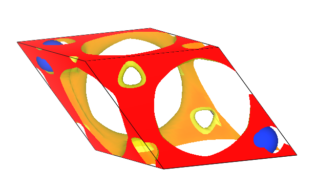
3vis_vol.py:1# coding:utf-8 2from dspawpy.io.write import write_VESTA 3 4# Read data file (in h5 or json format), process it, and output to a cube file 5write_VESTA( 6 in_filename="dspawpy_proj/dspawpy_tests/inputs/2.2/rho.h5", # Path to the json or h5 file containing electronic system information 7 data_type="rho", # Data type, supported values are "rho", "potential", "elf", "pcharge", "rhoBound" 8 out_filename="dspawpy_proj/dspawpy_tests/outputs/us/DS-PAW_rho.cube", # Output file path 9 gridsize=(10, 10, 10), # Specifies the interpolation grid size 10 format="cube", # Supported formats: cube, vesta, and txt (xyz grid coordinates + values) 11)
Drag the converted file DS-PAW_rho.cube into the VESTA software to visualize it:
Differential volumetric data visualization
See
3dvol.py:1# coding:utf-8 2from dspawpy.io.write import write_delta_rho_vesta 3 4# Read the data file (h5 or json format), process it, and output it to a cube file, which can be directly opened with Vesta and has a small volume 5write_delta_rho_vesta( 6 total="dspawpy_proj/dspawpy_tests/inputs/supplement/AB.h5", # Data file for the system containing all components 7 individuals=[ 8 "dspawpy_proj/dspawpy_tests/inputs/supplement/A.h5", 9 "dspawpy_proj/dspawpy_tests/inputs/supplement/B.h5", 10 ], # Data files for the system containing each component 11 output="dspawpy_proj/dspawpy_tests/outputs/us/3delta_rho.cube", # Output file path 12)
The above script supports the processing of charge density differences in multi-component systems. As an example using a binary system, it generates the charge density difference file delta_rho.cube from AB.h5, A.h5, and B.h5. This file can be directly opened using VESTA.
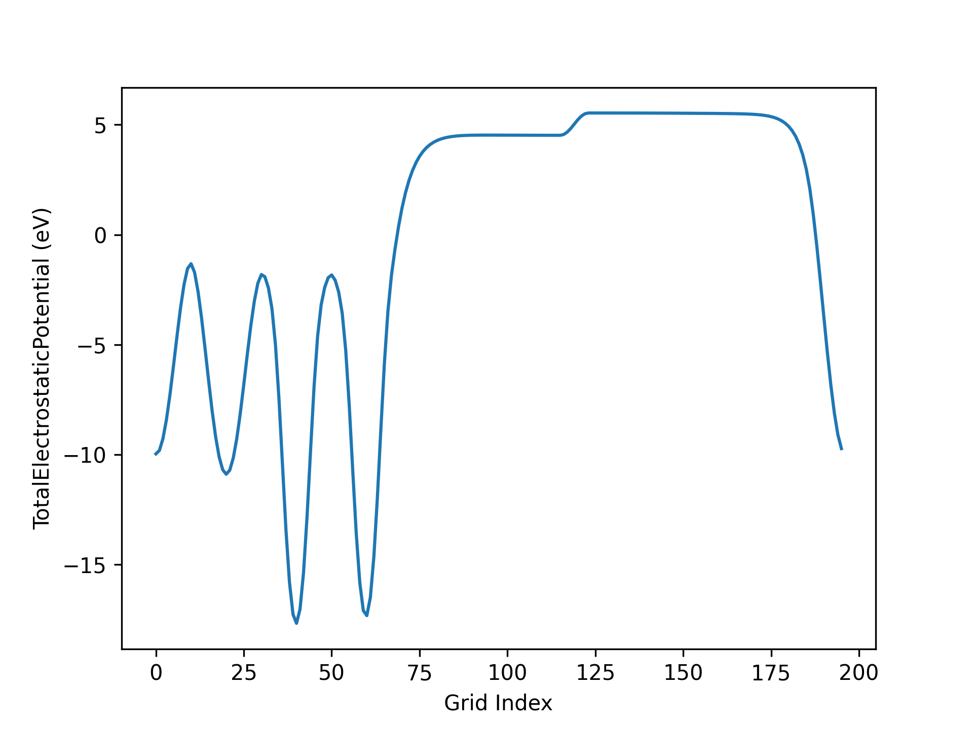
Volumetric data plane average
See also
3planar_ave.py:
 1# coding:utf-8
 2from dspawpy.plot import average_along_axis
 3
 4axes = [
 5    "2"
 6]  # "0", "1", "2" correspond to the x, y, z axes respectively; select which axes to average along
 7axes_indices = [int(i) for i in axes]
 8for ai in axes_indices:
 9    plt = average_along_axis(
10        datafile="dspawpy_proj/dspawpy_tests/inputs/3.3/scf.h5",  # Data file path
11        task="potential",  # Task name, can be 'rho', 'potential', 'elf', 'pcharge', 'rhoBound'
12        axis=ai,  # Axis along which to plot the potential curve
13        smooth=False,  # Whether to smooth
14        smooth_frac=0.8,  # Smoothing coefficient
15        subtype=None,  # Used to specify the subclass of task data, currently only used for Potential
16        label=f"axis{ai}",  # Legend label
17    )
18if len(axes_indices) > 1:
19    plt.legend()
20
21plt.xlabel("Grid Index")
22plt.ylabel("TotalElectrostaticPotential (eV)")
23plt.savefig("dspawpy_proj/dspawpy_tests/outputs/us/3pot_ave.png", dpi=300)  # Image name
Processing the electrostatic potential file obtained from Section 3.3 of Application Cases yields the following vacuum direction potential function curve:
警告
If you execute the above script by connecting to a remote server via SSH and encounter QT-related error messages, it’s possible that the program you are using (e.g., MobaXterm) is incompatible with the QT libraries. You should either switch programs (e.g., VSCode or the system’s built-in terminal command line) or add the following code, starting from the second line of your Python script:
import matplotlib
matplotlib.use('agg')
8.4 band data processing
备注
The script calls get_band_data() to read data, and setting efermi=XX during data reading can shift the energy zero point to the specified value; setting zero_to_efermi=True can shift the energy zero point to the Fermi level in the read file.
When plotting using pymatgen’s BSPlotter.get_plot() in the script, you can set zero_to_efermi=True to shift the energy zero to the Fermi level. Due to a critical update in pymatgen on August 17, 2023, which changed the return object of the plotting function from plt to axes, subsequent scripts may become incompatible. Therefore, a conditional statement has been added to handle this in the relevant parts of the user’s script.
For two-step band calculations, obtain the accurate Fermi level from the first-step self-consistent calculation (from the self-consistent system.json). If this fails, users can modify the energy zero point when calling get_band_data to read data, using the efermi parameter. For example: band_data=get_band_data(‘band.h5’,efermi=-1.5)
When plotting, the script calls BSPlotter.get_plot from pymatgen. When the system is determined to be non-metallic, setting zero_to_efermi will consider the VBM as the Fermi level energy, rather than the Fermi level from the data file. Therefore, when the system is non-metallic, setting zero_to_efermi=True during data reading and setting zero_to_efermi=True during plotting will result in different plots.
Running the Python script listed in this section, the program will determine whether the system is metallic. If it is a non-metallic system, you will be prompted to choose whether to shift the Fermi level to the zero energy point; please follow the prompts.
Conventional Band Treatment
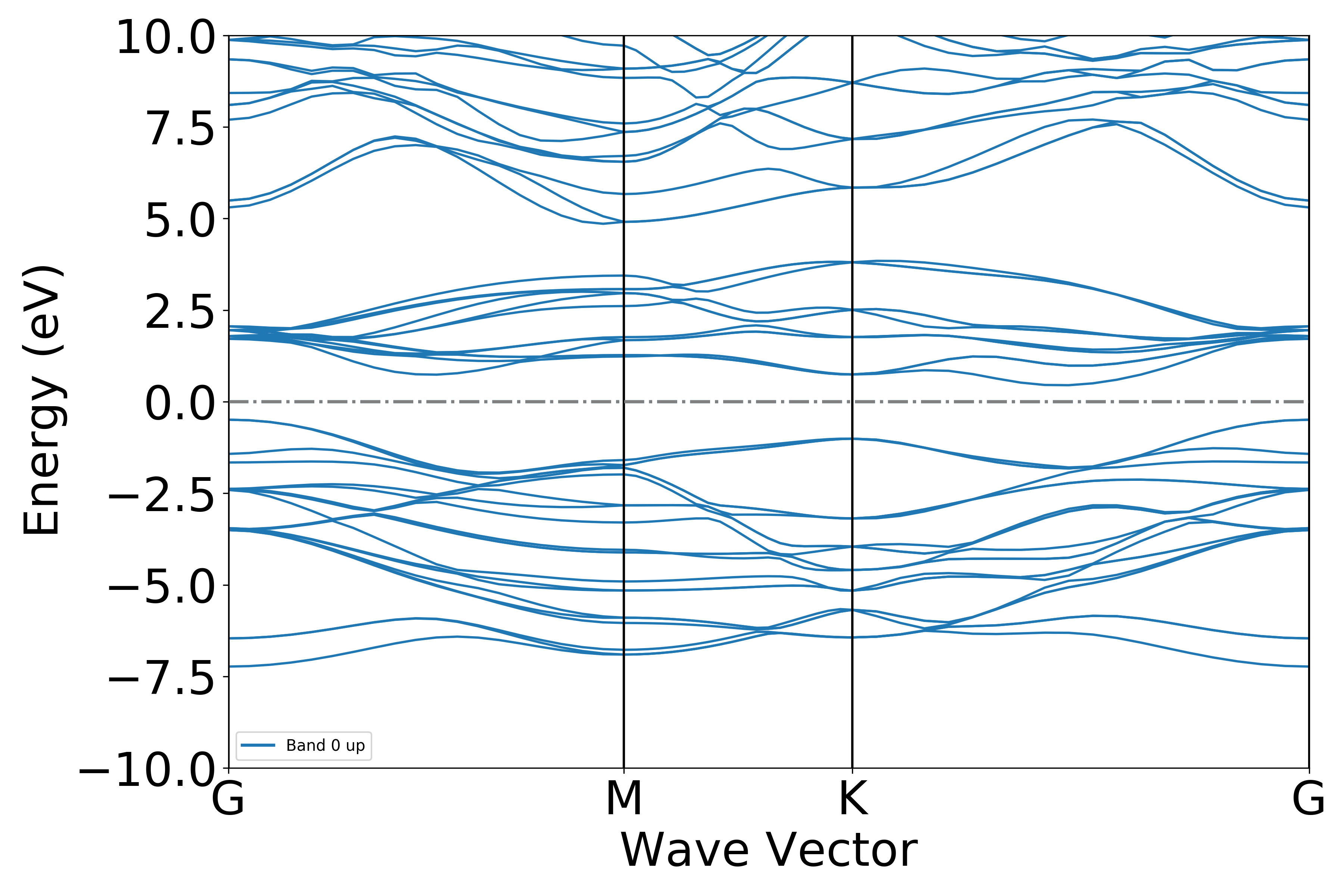
See 4bandplot.py:
 1# coding:utf-8
 2import os
 3import matplotlib.pyplot as plt
 4from pymatgen.electronic_structure.plotter import BSPlotter
 5
 6from dspawpy.io.read import get_band_data
 7
 8datafile = "dspawpy_proj/dspawpy_tests/inputs/supplement/pband.h5"  # Specifies the data file path
 9band_data = get_band_data(
10    band_dir=datafile,
11    syst_dir=None,  # path to system.json file, required only when band_dir is a json file
12    efermi=None,  # Used for manually correcting the Fermi level
13    zero_to_efermi=True,  # For non-metallic systems, the zero point energy should be shifted to the Fermi level
14)
15
16bsp = BSPlotter(band_data)
17axes_or_plt = bsp.get_plot(
18    zero_to_efermi=False,  # The data has already been shifted when read, so this should be turned off
19    ylim=[-10, 10],  # Range of the y-axis for the band structure plot
20    smooth=False,  # Whether to smooth the band structure plot
21    vbm_cbm_marker=False,  # Whether to mark the valence band maximum and conduction band minimum in the band structure plot
22    smooth_tol=0,  # Threshold for smoothing
23    smooth_k=3,  # Order of the smoothing process
24    smooth_np=100,  # Number of points for smoothing
25)
26
27if isinstance(axes_or_plt, plt.Axes):
28    fig = axes_or_plt.get_figure()  # version newer than v2023.8.10
29else:
30    fig = axes_or_plt.gcf()  # older version pymatgen
31
32# Add a reference line for the energy zero point
33for ax in fig.axes:
34    ax.axhline(0, lw=2, ls="-.", color="gray")
35
36figname = "dspawpy_proj/dspawpy_tests/outputs/us/4bandplot.png"  # Filename for the output band plot
37os.makedirs(os.path.dirname(os.path.abspath(figname)), exist_ok=True)
38fig.savefig(figname, dpi=300)
备注
For band structure calculations, an accurate Fermi level is required, which is obtained from the self-consistent calculation (from system.json). If the acquisition fails, users can modify the efermi parameter in the get_band_data function.
Executing the code will generate a band structure plot similar to the following:
The band is projected onto each element separately, with the size of the data points representing the element’s contribution to the orbital.
See 4bandplot_elt.py:
 1# coding:utf-8
 2import os
 3
 4import matplotlib.pyplot as plt
 5import numpy as np
 6from pymatgen.electronic_structure.plotter import BSPlotterProjected
 7
 8from dspawpy.io.read import get_band_data
 9
10datafile = "dspawpy_proj/dspawpy_tests/inputs/supplement/pband.h5"  # Specify the data file path
11band_data = get_band_data(
12    band_dir=datafile,
13    syst_dir=None,  # path to system.json file, required only when band_dir is a json file
14    efermi=None,  # Used to manually adjust the Fermi level
15    zero_to_efermi=True,  # For non-metallic systems, shift the zero-point energy to the Fermi level
16)
17
18bsp = BSPlotterProjected(bs=band_data)  # Initialize the BSPlotterProjected class
19axes_or_plt = bsp.get_elt_projected_plots(
20    zero_to_efermi=False,  # The data has already been shifted when read, so this should be disabled
21    ylim=[-8, 5],  # Set the energy range
22    vbm_cbm_marker=False,  # Whether to mark the conduction band minimum (CBM) and valence band maximum (VBM)
23)
24
25if isinstance(axes_or_plt, plt.Axes):
26    fig = axes_or_plt.get_figure()  # version newer than v2023.8.10
27elif np.iterable(axes_or_plt):
28    fig = np.asarray(axes_or_plt).flatten()[0].get_figure()
29else:
30    fig = axes_or_plt.gcf()  # older version pymatgen
31
32# Add a reference line for the energy zero point
33for ax in fig.axes:
34    ax.axhline(0, lw=2, ls="-.", color="gray")
35
36figname = "dspawpy_proj/dspawpy_tests/outputs/us/4bandplot_elt.png"  # The filename for the output band plot
37os.makedirs(os.path.dirname(os.path.abspath(figname)), exist_ok=True)
38fig.savefig(figname, dpi=300)
备注
To plot projected band structure data, use the BSPlotterProjected module.
Use the get_elt_projected_plots function in the BSPlotterProjected module to plot band diagrams with orbital contributions for each element.
Executing the code will generate band plots similar to the following:
警告
If you execute the script above by connecting to a remote server via SSH, and you encounter QT-related error messages, it’s possible that the program you’re using (such as MobaXterm) is incompatible with the QT libraries. You can either switch to a different program (e.g., VSCode or the system’s built-in terminal command line), or add the following code, starting on the second line of your Python script:
import matplotlib
matplotlib.use('agg')
Band projections onto different elements’ different orbitals
Refer to 4bandplot_elt_orbit.py:
 1# coding:utf-8
 2import os
 3
 4import matplotlib.pyplot as plt
 5import numpy as np
 6from pymatgen.electronic_structure.plotter import BSPlotterProjected
 7
 8from dspawpy.io.read import get_band_data
 9
10datafile = "dspawpy_proj/dspawpy_tests/inputs/supplement/pband.h5"  # Specify the data file path
11band_data = get_band_data(
12    band_dir=datafile,
13    syst_dir=None,  # path to system.json file, only required when band_dir is a json file
14    efermi=None,  # Used for manually correcting the Fermi level
15    zero_to_efermi=True,  # For non-metallic systems, shift the zero point energy to the Fermi level
16)
17
18bsp = BSPlotterProjected(bs=band_data)  # Initialize the BSPlotterProjected class
19# Select elements and orbitals, create a dictionary
20dict_elem_orbit = {"Mo": ["d"], "S": ["s"]}
21
22axes_or_plt = bsp.get_projected_plots_dots(
23    dictio=dict_elem_orbit,
24    zero_to_efermi=False,  # The data has already been shifted when read, so this should be turned off
25    ylim=[-8, 5],  # Set the energy range
26    vbm_cbm_marker=False,  # Whether to mark the conduction band minimum and valence band maximum
27)
28
29if isinstance(axes_or_plt, plt.Axes):
30    fig = axes_or_plt.get_figure()  # version newer than v2023.8.10
31elif np.iterable(axes_or_plt):
32    fig = np.asarray(axes_or_plt).flatten()[0].get_figure()
33else:
34    fig = axes_or_plt.gcf()  # older version pymatgen
35
36# Add a reference line for the energy zero point
37for ax in fig.axes:
38    ax.axhline(0, lw=2, ls="-.", color="gray")
39
40figname = "dspawpy_proj/dspawpy_tests/outputs/us/4bandplot_elt_orbit.png"  # Filename for the output band plot
41os.makedirs(os.path.dirname(os.path.abspath(figname)), exist_ok=True)
42fig.savefig(figname, dpi=300)
备注
Use the get_projected_plots_dots method in the BSPlotterProjected module, which allows users to customize the band structure plots by specifying elements and orbitals (L) to be plotted.
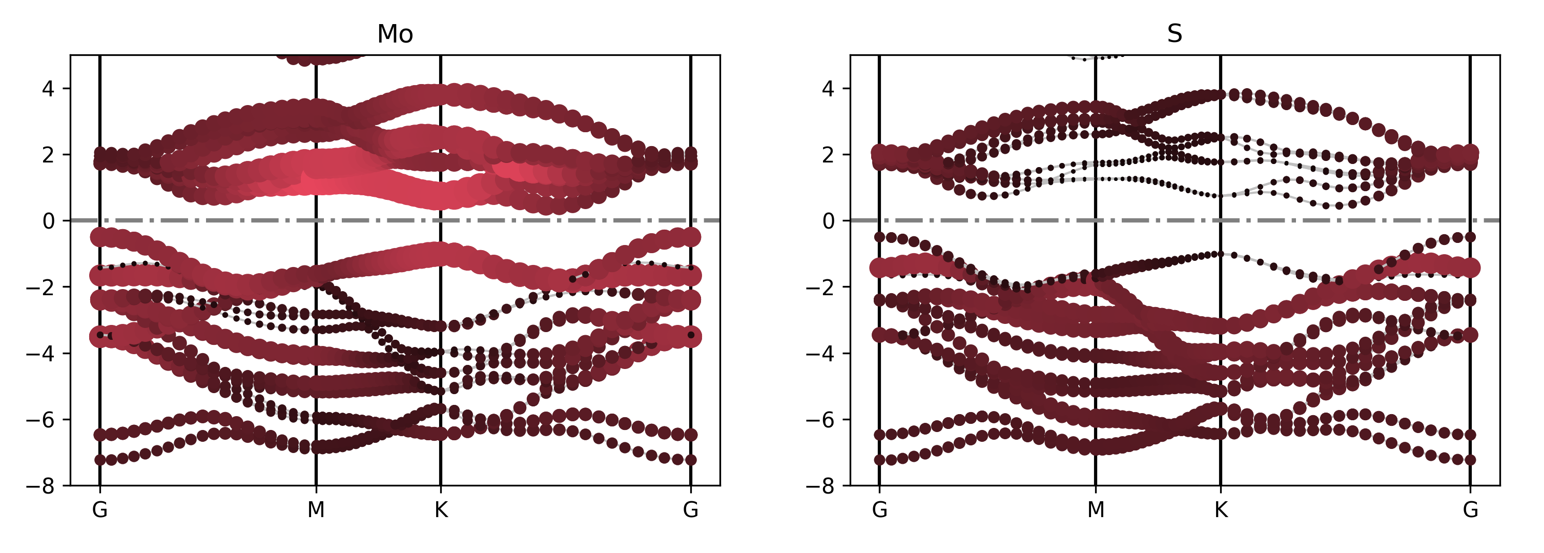
For example, get_projected_plots_dots({‘Mo’: [‘d’], ‘S’: [‘s’]}) plots the d-orbitals of Mo and the s-orbitals of S.
Executing the code will generate a band structure plot similar to the following:
警告
If you execute the above script by connecting to a remote server via SSH, and QT-related error messages appear, it may be due to incompatibility between the program used (e.g., MobaXterm) and the QT library. Either change the program (e.g., VSCode or the system’s built-in terminal command line), or add the following code starting from the second line of your Python script:
import matplotlib
matplotlib.use('agg')
Projecting band structure onto different atomic orbitals
See 4bandplot_patom_porbit.py:
 1# coding:utf-8
 2import os
 3
 4import matplotlib.pyplot as plt
 5import numpy as np
 6from pymatgen.electronic_structure.plotter import BSPlotterProjected
 7
 8from dspawpy.io.read import get_band_data
 9
10datafile = "dspawpy_proj/dspawpy_tests/inputs/supplement/pband.h5"  # Specify the data file path
11band_data = get_band_data(
12    band_dir=datafile,
13    syst_dir=None,  # path to system.json file, required only when band_dir is a JSON file
14    efermi=None,  # Used to manually adjust the Fermi level
15    zero_to_efermi=True,  # For non-metallic systems, shift the zero point energy to the Fermi level
16)
17
18bsp = BSPlotterProjected(bs=band_data)
19# Specify elements, orbitals, and atomic numbers
20dict_elem_orbit = {"Mo": ["px", "py", "pz"]}
21dict_elem_index = {"Mo": [1]}
22
23axes_or_plt = bsp.get_projected_plots_dots_patom_pmorb(
24    dictio=dict_elem_orbit,  # Specify the element-orbit dictionary
25    dictpa=dict_elem_index,  # Specify the element-atomic number dictionary
26    sum_atoms=None,  # Whether to sum over atoms
27    sum_morbs=None,  # Whether to sum orbitals
28    zero_to_efermi=False,  # Data has already been shifted during reading, should be turned off here
29    ylim=None,  # Set the energy range
30    vbm_cbm_marker=False,  # Whether to mark the conduction band minimum and valence band maximum
31    selected_branches=None,  # Specify the energy band branches to be plotted
32    w_h_size=(12, 8),  # Set image width and height
33    num_column=None,  # Number of images displayed per row
34)
35
36if isinstance(axes_or_plt, plt.Axes):
37    fig = axes_or_plt.get_figure()  # version newer than v2023.8.10
38elif np.iterable(axes_or_plt):
39    fig = np.asarray(axes_or_plt).flatten()[0].get_figure()
40else:
41    fig = axes_or_plt.gcf()  # older version pymatgen
42
43# Add a reference line for the energy zero point
44for ax in fig.axes:
45    ax.axhline(0, lw=2, ls="-.", color="gray")
46
47figname = " dspawpy_proj/dspawpy_tests/outputs/us/4band_patom_porbit.png"  # Output bandpass figure filename
48os.makedirs(os.path.dirname(os.path.abspath(figname)), exist_ok=True)
49fig.savefig(figname, dpi=300)
备注
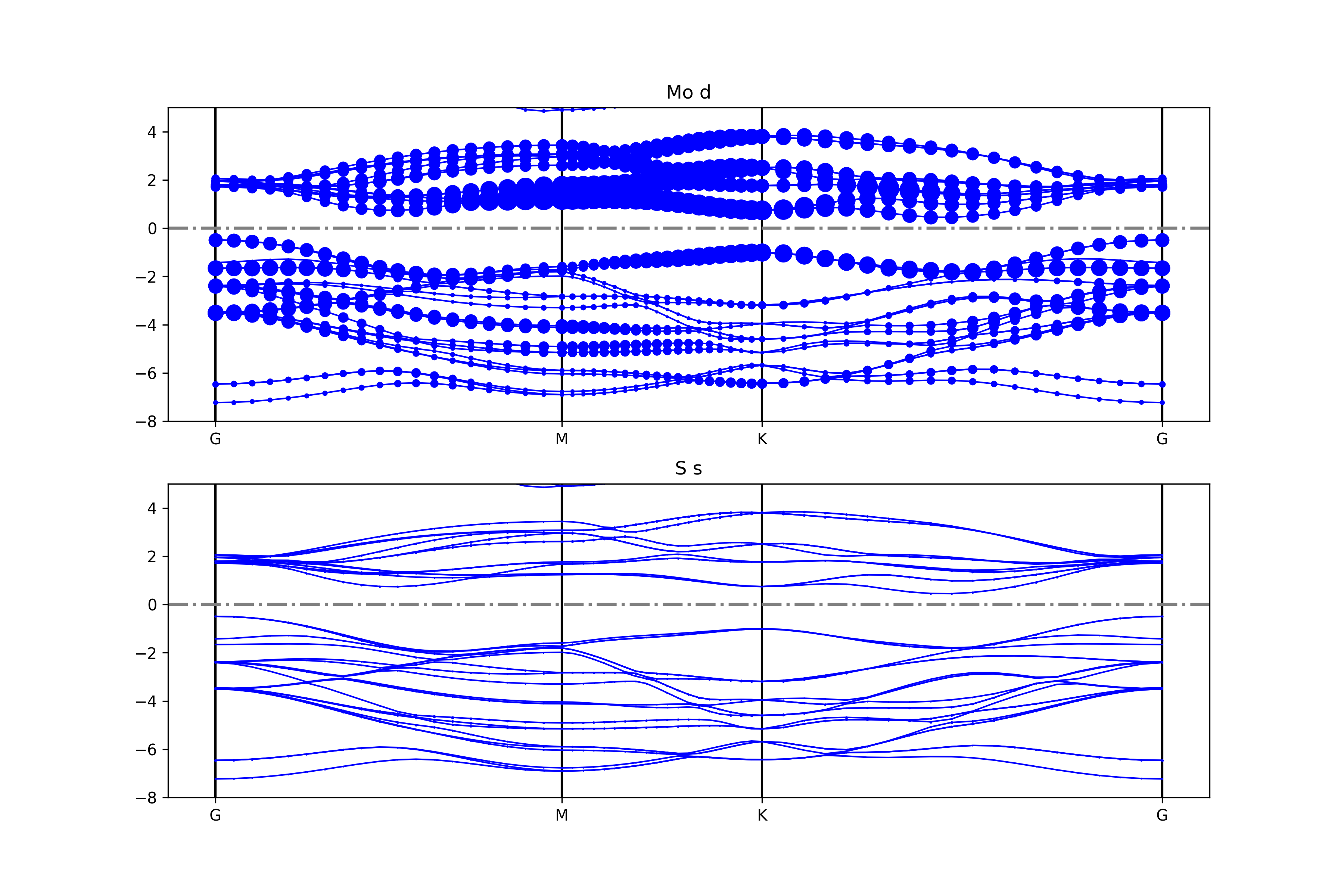
The get_projected_plots_dots_patom_pmorb function in the BSPlotterProjected module offers greater flexibility, allowing users to customize the band diagrams for specific atoms and orbitals.
Use dictpa to specify the atom, and dictio to specify the orbitals of that atom.
To superimpose projected components of some atoms or orbitals, specify the sum_atoms or sum_morbs parameters according to the documentation of the get_projected_plots_dots_patom_pmorb function.
警告
If only a single orbital is selected and the orbital name has more than one letter (e.g., px, dxy, dxz), the get_projected_plots_dots_patom_pmorb function will raise an error. See here for details.
Executing the code will generate band diagrams similar to the following:
警告
If you execute the above script by connecting to a remote server via SSH, and you encounter QT-related error messages, it’s possible that the program you’re using (e.g., MobaXterm) is incompatible with the QT libraries. Either switch to another program (e.g., VSCode or the system’s built-in terminal command line), or add the following code starting from the second line of your Python script:
import matplotlib
matplotlib.use('agg')
Band unfolding processing
See 4bandunfolding.py:
 1# coding:utf-8
 2import os
 3
 4from dspawpy.plot import plot_bandunfolding
 5
 6plt = plot_bandunfolding(
 7    datafile="dspawpy_proj/dspawpy_tests/inputs/2.22.1/band.h5",  # Read data
 8    ef=None,  # Fermi level, read from the file
 9    de=0.05,  # Band width, default 0.05
10    dele=0.06,  # Band gap, default 0.06
11)
12
13plt.ylim(-15, 10)
14figname = "dspawpy_proj/dspawpy_tests/outputs/us/4bandunfolding.png"  # Output band structure plot filename
15os.makedirs(os.path.dirname(os.path.abspath(figname)), exist_ok=True)
16plt.savefig(figname, dpi=300)
17# plt.show()
Executing the code yields a band diagram similar to the following:

警告
警告
This feature currently does not support setting the Fermi level of non-metallic materials as the zero-energy point (the default is the valence band top as the zero-energy point).
警告
If you execute the above script by connecting to a remote server via SSH and encounter QT-related error messages, it might be due to incompatibility between the program used (such as MobaXterm, etc.) and the QT library. You can either switch programs (e.g., VSCode or the system’s built-in terminal) or add the following code starting from the second line of your Python script:
import matplotlib
matplotlib.use('agg')
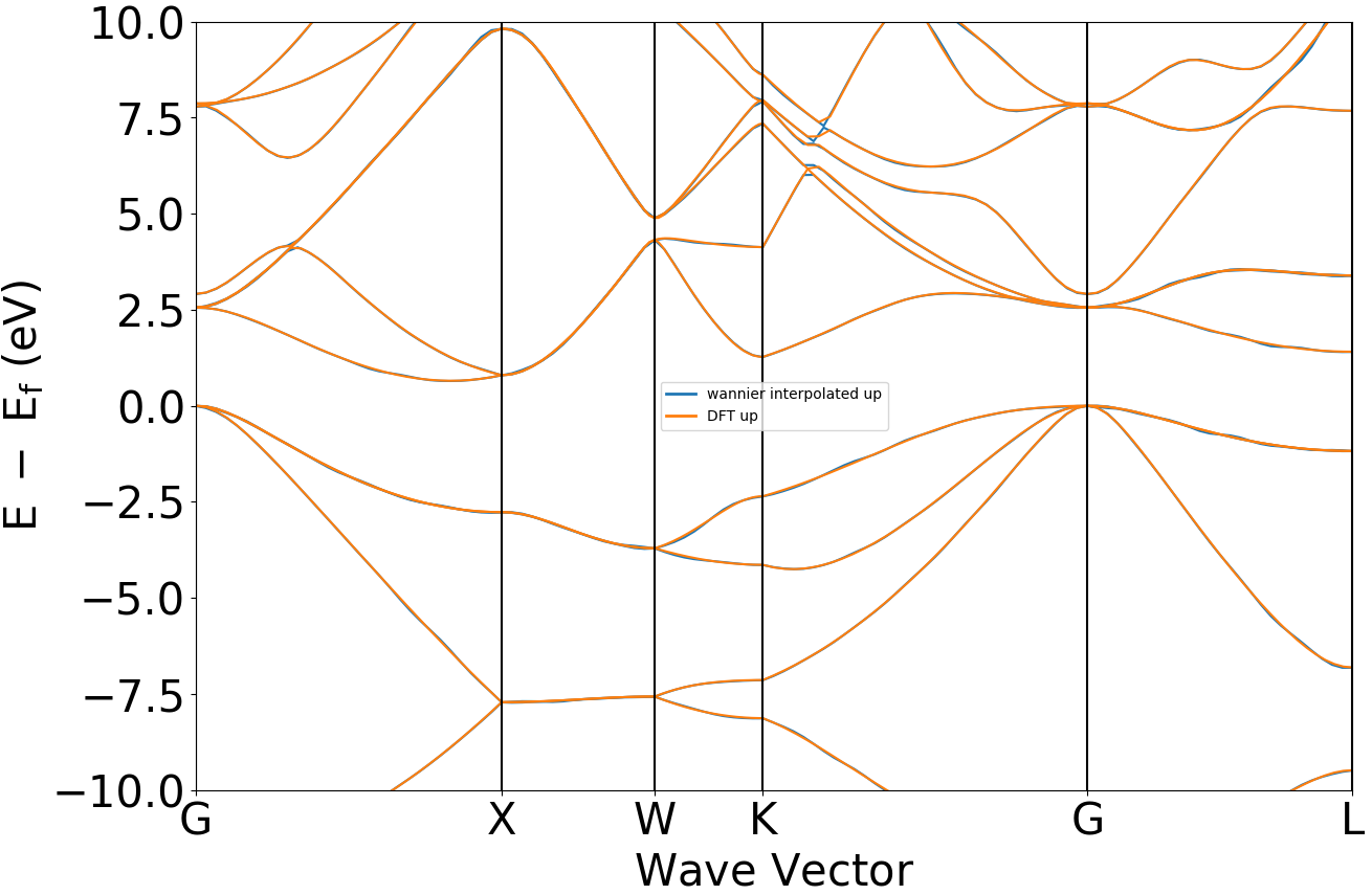
band-compare band structure comparison figure processing
Plotting regular band structure and Wannier band structure on the same figure.
Refer to 4bandcompare.py:
 1# coding:utf-8
 2import os
 3
 4from pymatgen.electronic_structure.plotter import BSPlotter
 5
 6from dspawpy.io.read import get_band_data
 7
 8band_data = get_band_data(
 9    band_dir="dspawpy_proj/dspawpy_tests/inputs/2.30/wannier.h5",  # Wannier band file path
10    syst_dir=None,  # system.json file path, only needed when band_dir is a json file
11    efermi=None,  # Used for manually adjusting the Fermi level
12    zero_to_efermi=False,  # Whether to shift zero energy to the Fermi level
13)
14bsp = BSPlotter(bs=band_data)
15band_data = get_band_data(
16    band_dir="dspawpy_proj/dspawpy_tests/inputs/2.3/band.h5",  # Read DFT band structure
17    syst_dir=None,  # path to system.json file, required only when band_dir is a json file
18    efermi=None,  # Used for manually correcting the Fermi level
19    zero_to_efermi=False,  # Whether to shift the zero point energy to the Fermi level
20)
21
22bsp2 = BSPlotter(bs=band_data)
23bsp.add_bs(bsp2._bs)
24axes_or_plt = bsp.get_plot(
25    zero_to_efermi=True,  # Move the zero energy level to the Fermi level
26    ylim=[-10, 10],  # Energy band plot y-axis range
27    smooth=False,  # Whether to smooth the band structure plot
28    vbm_cbm_marker=False,  # Whether to mark the valence band maximum and conduction band minimum in the band structure plot
29    smooth_tol=0,  # Threshold for smoothing
30    smooth_k=3,  # Order of the smoothing process
31    smooth_np=100,  # Number of points for smoothing
32    bs_labels=["wannier interpolated", "DFT"],  # Band structure labels
33)
34
35import matplotlib.pyplot as plt  # noqa: E402
36
37if isinstance(axes_or_plt, plt.Axes):
38    fig = axes_or_plt.get_figure()  # version newer than v2023.8.10
39else:
40    fig = axes_or_plt.gcf()  # older version pymatgen
41
42# Add a reference line for the energy zero point
43for ax in fig.axes:
44    ax.axhline(0, lw=2, ls="-.", color="gray")
45
46figname = "dspawpy_proj/dspawpy_tests/outputs/us/4wanierBand.png"  # File name for the output band structure plot
47os.makedirs(os.path.dirname(os.path.abspath(figname)), exist_ok=True)
48fig.savefig(figname, dpi=300)
Executing the code will generate band comparison curves similar to the following:
警告
If you are running the above script by connecting to a remote server via SSH and encounter QT-related error messages, it may be due to incompatibility between the program you are using (such as MobaXterm, etc.) and the QT libraries. You can either switch to another program (such as VSCode or the system’s built-in terminal), or add the following code, starting from the second line of your Python script:
import matplotlib
matplotlib.use('agg')
8.5 DOS Data Processing
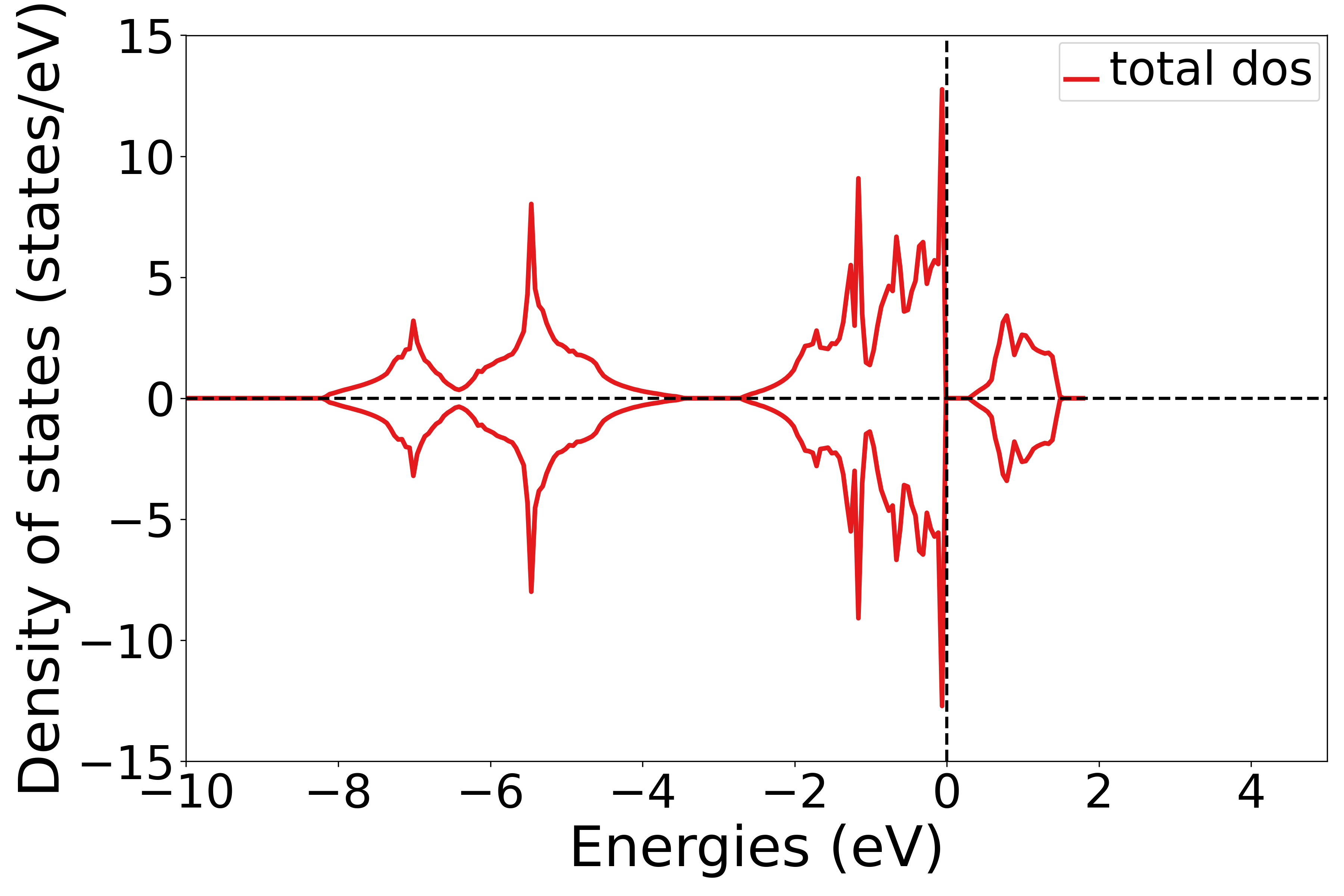
Total Density of States
See 5dosplot_total.py:
 1# coding:utf-8
 2import os
 3
 4from pymatgen.electronic_structure.plotter import DosPlotter
 5
 6from dspawpy.io.read import get_dos_data
 7from dspawpy.plot import plot_dos
 8
 9dos_data = get_dos_data(
10    dos_dir="dspawpy_proj/dspawpy_tests/inputs/3.2.4/dos.h5",  # Read projected density of states data
11    return_dos=False,  # If False, always return a CompleteDos object (regardless of whether projection was enabled during calculation)
12)
13dos_plotter = DosPlotter(
14    zero_at_efermi=True,  # Whether to set the Fermi level as the zero point
15    stack=False,  # True indicates drawing an area chart
16    sigma=None,  # Gaussian broadening, None indicates no smoothing process
17)
18dos_plotter.add_dos(
19    label="total dos", dos=dos_data
20)  # Set the legend for the density of states plot  # Pass the density of states data
21
22ax = plot_dos(
23    dosplotter=dos_plotter,
24    xlim=[-10, 5],  # Set the energy range
25    ylim=[-15, 15],  # Set the density of states range
26)
27ax.axhline(0, lw=2, ls="-.", color="gray")
28
29filename = "dspawpy_proj/dspawpy_tests/outputs/us/5dos_total.png"  # File name for the output density of states plot
30os.makedirs(os.path.dirname(os.path.abspath(filename)), exist_ok=True)
31
32fig = ax.get_figure()
33fig.savefig(filename, dpi=300)
备注
Use the get_dos_data function to convert the dos.h5 file obtained from DS-PAW calculations into a format supported by pymatgen.
Use the DosPlotter module to obtain the data from the DS-PAW calculated dos.h5 file.
The DosPlotter function can pass parameters: the stack parameter indicates whether to fill the DOS plots, and zero_at_efermi indicates whether to set the Fermi energy to zero in the DOS plot. Here, stack=False and zero_at_efermi=False are set.
Use add_dos in the DosPlotter module to add the DOS data.
Use the get_plot function in the DosPlotter module to plot the DOS.
Executing the code will generate a density of states plot similar to the following:
警告
If you execute the above script by connecting to a remote server via SSH and encounter QT-related error messages, it’s likely that the program you’re using (such as MobaXterm, etc.) is incompatible with the QT libraries. You can either switch programs (e.g., VSCode or the system’s built-in terminal command line), or add the following code starting from the second line of your Python script:
import matplotlib
matplotlib.use('agg')
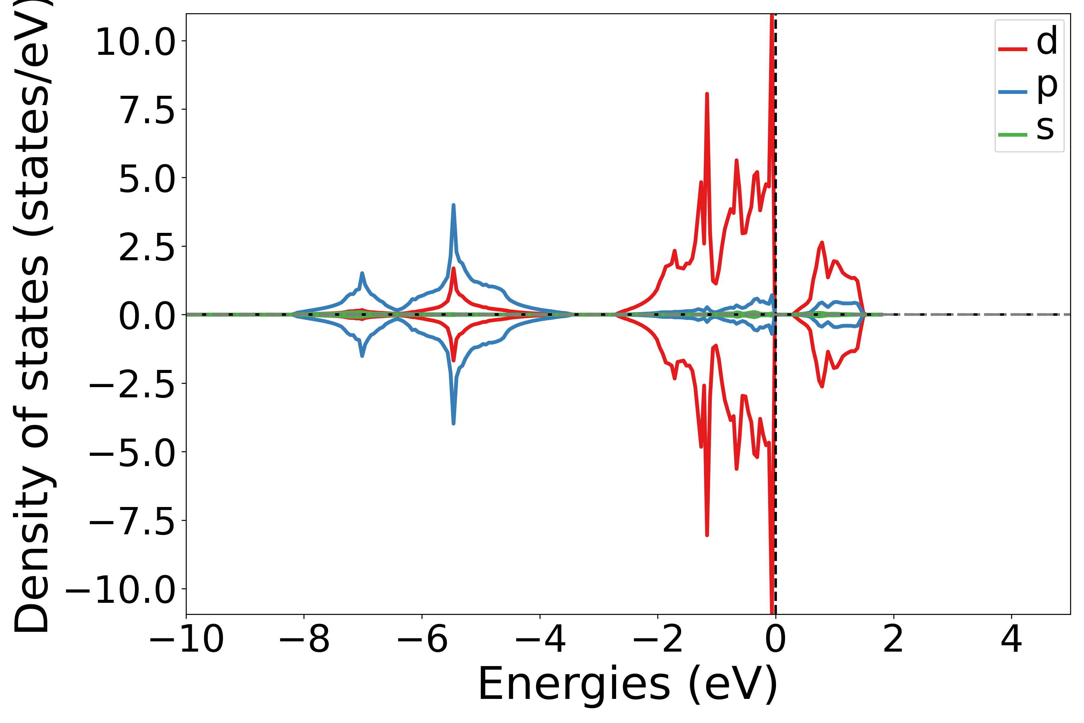
Project Density of States onto different orbitals
See 5dosplot_spd.py:
 1# coding:utf-8
 2import os
 3
 4from pymatgen.electronic_structure.plotter import DosPlotter
 5
 6from dspawpy.io.read import get_dos_data
 7from dspawpy.plot import plot_dos
 8
 9dos_data = get_dos_data(
10    dos_dir="dspawpy_proj/dspawpy_tests/inputs/3.2.4/dos.h5",  # Read projected DOS data
11    return_dos=False,  # If False, always return a CompleteDos object (regardless of whether projection was enabled during calculation)
12)
13dos_plotter = DosPlotter(
14    zero_at_efermi=True,  # Whether to set the Fermi level as the zero point
15    stack=False,  # True indicates drawing an area chart
16    sigma=None,  # Gaussian broadening, None indicates no smoothing is applied
17)
18dos_plotter.add_dos_dict(
19    dos_dict=dos_data.get_spd_dos(),
20    key_sort_func=None,  # Orbital projection  # Specifies the sorting function
21)
22ax = plot_dos(
23    dosplotter=dos_plotter,
24    xlim=[-10, 5],  # Set the energy range
25    ylim=None,  # Set the density of states range
26)
27
28ax.axhline(0, lw=2, ls="-.", color="gray")
29
30filename = "dspawpy_proj/dspawpy_tests/outputs/us/5dos_spd.png"  # Filename of the output density of states plot
31os.makedirs(os.path.dirname(os.path.abspath(filename)), exist_ok=True)
32
33fig = ax.get_figure()
34fig.savefig(filename, dpi=300)
备注
Use the add_dos_dict function in the DosPlotter module to obtain the projected density of states (DOS) data, and then use get_spd_dos to project the information onto spd orbitals.
The code execution will produce a density of states plot similar to the following:
警告
If you encounter QT-related error messages when executing the above script via SSH connection to a remote server, it might be due to incompatibility between the program used (e.g., MobaXterm) and the QT library. Either change the program (e.g., VSCode or the system’s built-in terminal command line), or add the following code starting from the second line of your Python script:
import matplotlib
matplotlib.use('agg')
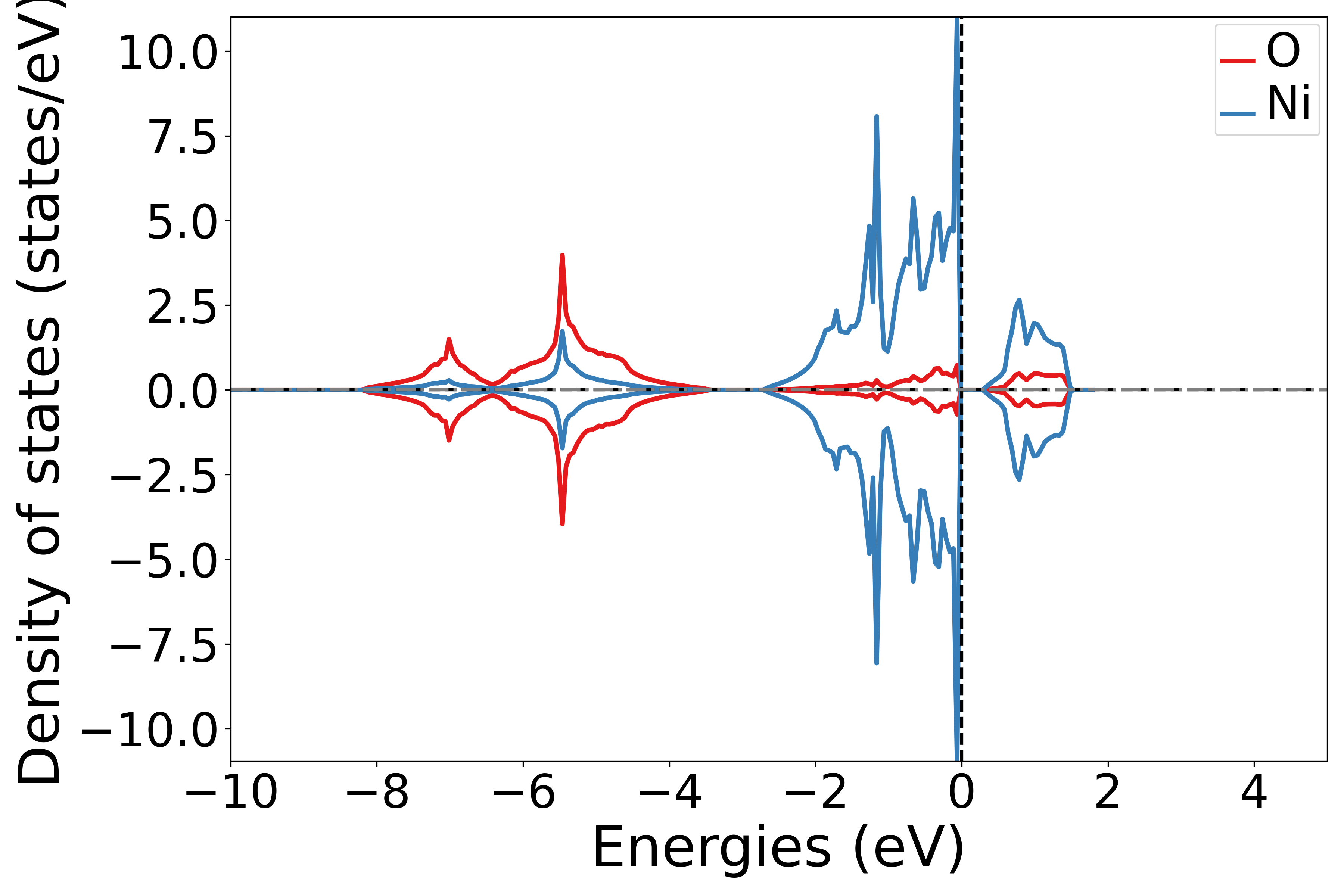
Projecting the density of states onto different elements
See also 5dosplot_elt.py:
 1# coding:utf-8
 2import os
 3
 4from pymatgen.electronic_structure.plotter import DosPlotter
 5
 6from dspawpy.io.read import get_dos_data
 7from dspawpy.plot import plot_dos
 8
 9dos_data = get_dos_data(
10    dos_dir="dspawpy_proj/dspawpy_tests/inputs/3.2.4/dos.h5",  # Reads projected DOS data
11    return_dos=False,  # If False, always returns a CompleteDos object (regardless of whether projection was enabled during calculation)
12)
13dos_plotter = DosPlotter(
14    zero_at_efermi=True,  # Whether to set the Fermi level as the zero point
15    stack=False,  # True indicates drawing an area chart
16    sigma=None,  # Gaussian broadening, None indicates no smoothing is applied
17)
18dos_plotter.add_dos_dict(
19    dos_dict=dos_data.get_element_dos(),
20    key_sort_func=None,  # Projected DOS for elements  # Specify the sorting function
21)
22
23ax = plot_dos(
24    dosplotter=dos_plotter,
25    xlim=[-10, 5],  # Set the energy range
26    ylim=None,  # Set the density of states range
27)
28ax.axhline(0, lw=2, ls="-.", color="gray")
29
30filename = "dspawpy_proj/dspawpy_tests/outputs/us/5dos_elt.png"  # Filename for the output density of states plot
31os.makedirs(os.path.dirname(os.path.abspath(filename)), exist_ok=True)
32
33fig = ax.get_figure()
34fig.savefig(filename, dpi=300)
备注
Use the add_dos_dict function in the DosPlotter module to obtain projected density of states data, then use get_element_dos to output the projected information according to different elements.
The code execution will produce a density of states plot similar to the following:
警告
If you encounter QT-related error messages when executing the above script via SSH connection to a remote server, it might be due to incompatibility between the program used (e.g., MobaXterm) and the QT library. Either change the program (e.g., VSCode or the system’s built-in terminal command line), or add the following code starting from the second line of your Python script:
import matplotlib
matplotlib.use('agg')
Projecting the density of states onto different orbitals of different atoms
 1# coding:utf-8
 2import os
 3
 4from pymatgen.electronic_structure.core import Orbital
 5from pymatgen.electronic_structure.plotter import DosPlotter
 6
 7from dspawpy.io.read import get_dos_data
 8from dspawpy.plot import plot_dos
 9
10dos_data = get_dos_data(
11    dos_dir="dspawpy_proj/dspawpy_tests/inputs/3.2.4/dos.h5",  # Reads projected density of states data
12    return_dos=False,  # If False, always return a CompleteDos object (regardless of whether projection was enabled during calculation)
13)
14dos_plotter = DosPlotter(
15    zero_at_efermi=True,  # Whether to set the Fermi level as the zero point
16    stack=False,  # True indicates drawing an area plot
17    sigma=None,  # Gaussian broadening, None indicates no smoothing treatment
18)
19
20# ! Specify atomic number and orbital
21dict_index_orbit = {0: ["dxy"], 2: ["s"]}
22
23print("Plotting...")
24for index in dict_index_orbit:
25    _os = dict_index_orbit[index]
26    _e = str(dos_data.structure.sites[index].species)
27    for _orb in _os:
28        dos_plotter.add_dos(
29            f"{_e}(atom-{index}) {_orb}",  # label
30            dos_data.get_site_orbital_dos(
31                dos_data.structure[index],
32                getattr(Orbital, _orb),
33            ),
34        )
35
36ax = plot_dos(
37    dosplotter=dos_plotter,
38    xlim=[-10, 5],  # Set the energy range
39    ylim=None,  # Set the density of states range
40)
41ax.axhline(0, lw=2, ls="-.", color="gray")
42
43figname = "dspawpy_proj/dspawpy_tests/outputs/us/5dos_atom_orbit.png"  # Output density of states figure filename
44os.makedirs(os.path.dirname(os.path.abspath(figname)), exist_ok=True)
45
46fig = ax.get_figure()
47fig.savefig(figname, dpi=300)
备注
Use the get_site_orbital_dos function to extract the contribution of a specific atom and specific orbital from the DOS data. dos_data.structure[0], Orbital(4) represents obtaining the density of states for the dxy orbital of the first atom; the index in the get_site_orbital_dos function starts from 0.
Running this script and selecting the element and orbital as prompted will generate the corresponding density of states (DOS) plot.
Executing the code will produce a density of states plot similar to the following:
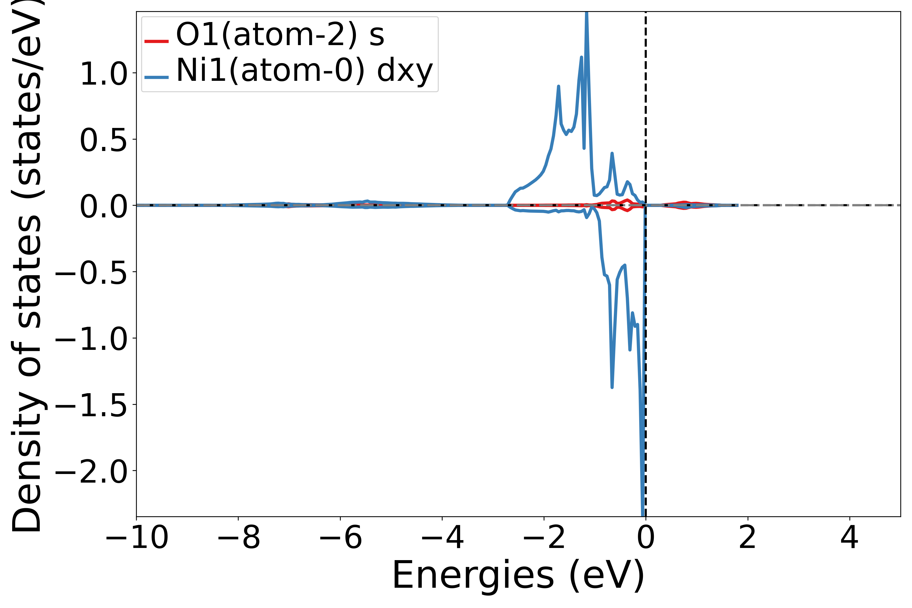
警告
If you encounter QT-related error messages when executing the above script via SSH connection to a remote server, it’s likely due to incompatibility between the program you’re using (e.g., MobaXterm) and the QT library. Either switch to a different program (such as VSCode or the system’s built-in terminal command line), or add the following code to your Python script starting from the second line:
import matplotlib
matplotlib.use('agg')
Projecting the density of states onto the split d-orbitals (t2g, eg) of different atoms
See also 5dosplot_t2g_eg.py:
 1# coding:utf-8
 2import os
 3
 4from pymatgen.electronic_structure.plotter import DosPlotter
 5
 6from dspawpy.io.read import get_dos_data
 7from dspawpy.plot import plot_dos
 8
 9dos_data = get_dos_data(
10    dos_dir="dspawpy_proj/dspawpy_tests/inputs/3.2.4/dos.h5",  # Read projected density of states data
11    return_dos=False,  # If False, always returns a CompleteDos object (regardless of whether projection was enabled during calculation)
12)
13dos_plotter = DosPlotter(
14    zero_at_efermi=True,  # Whether to set the Fermi level as the zero point
15    stack=False,  # True indicates drawing an area chart
16    sigma=None,  # Gaussian broadening, None indicates no smoothing is applied
17)
18# print(dos_data.structure)
19
20# Specify the atomic number, starting from 0
21ais = [1]
22
23print("Plotting...")
24atom_indices = [int(ai) for ai in ais]
25for atom_index in atom_indices:
26    dos_plotter.add_dos_dict(
27        dos_data.get_site_t2g_eg_resolved_dos(dos_data.structure[atom_index]),
28    )
29
30ax = plot_dos(
31    dosplotter=dos_plotter,
32    xlim=[-10, 5],  # Set the energy range
33    ylim=None,  # Set the density of states range
34)
35ax.axhline(0, lw=2, ls="-.", color="gray")
36
37filename = "dspawpy_proj/dspawpy_tests/outputs/us/5dos_t2g_eg.png"  # Output density of states plot filename
38os.makedirs(os.path.dirname(os.path.abspath(filename)), exist_ok=True)
39
40fig = ax.get_figure()
41fig.savefig(filename, dpi=300)
备注
Use the get_site_t2g_eg_resolved_dos function to extract the t2g and eg orbital contributions for a specific atom from the DOS data. This retrieves the t2g and eg orbital contributions for the second atom.
Running this script and selecting an atom number as prompted will generate the corresponding density of states plot.
Executing the code will generate a density of states plot similar to the following:
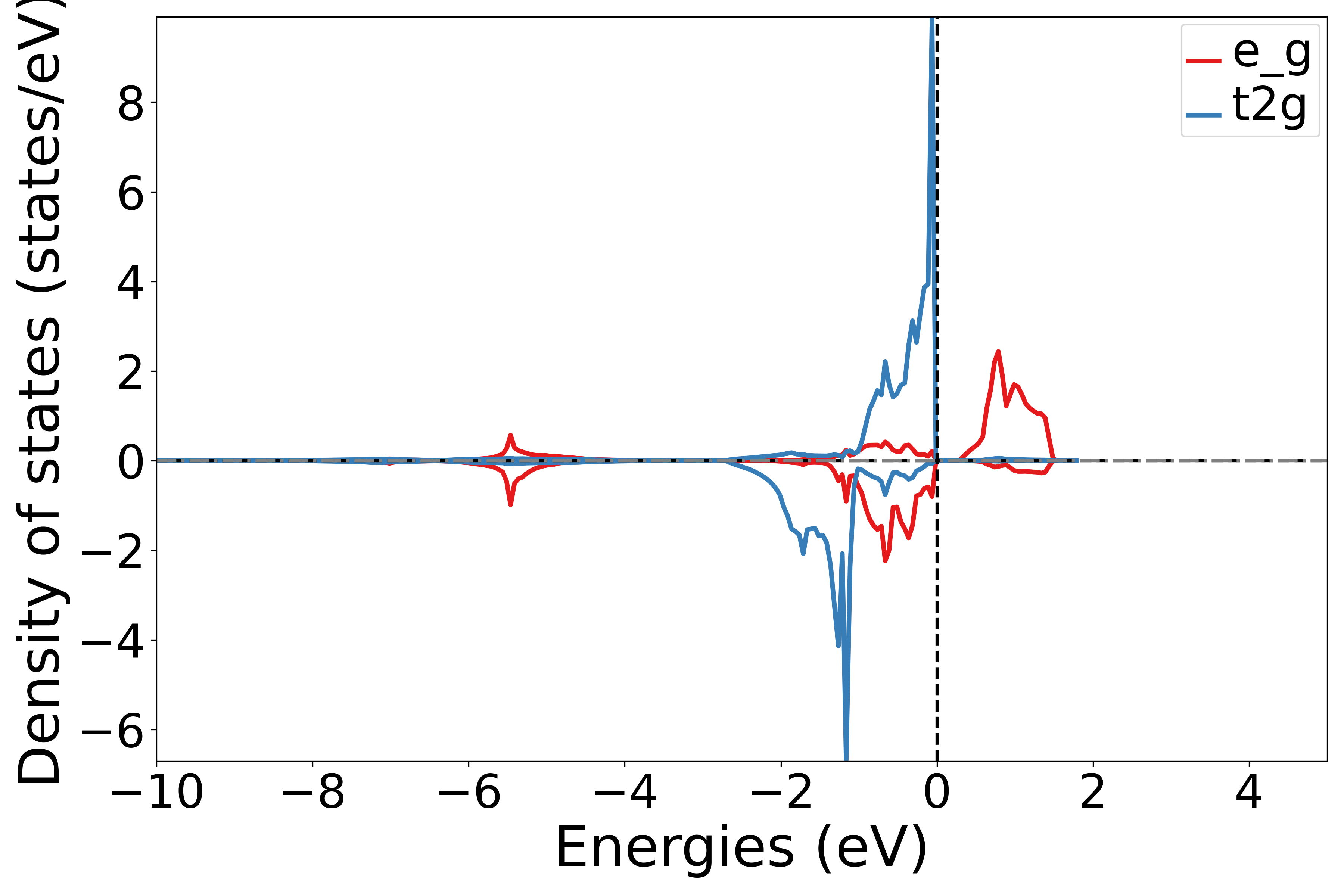
备注
If the element does not contain d orbitals, a blank image will be drawn.
警告
If you execute the script above by connecting to a remote server via SSH and encounter QT-related error messages, it’s likely that the program you are using (such as MobaXterm) is incompatible with the QT library. You can either switch programs (e.g., VSCode or the system’s built-in terminal command line) or add the following code starting from the second line of your Python script:
import matplotlib
matplotlib.use('agg')
d-centered analysis
Taking the Pb-slab system as an example, a d-band center analysis is performed on Pt atoms:
See 5center_dband.py:
 1# coding:utf-8
 2from dspawpy.io.read import get_dos_data
 3from dspawpy.io.utils import d_band
 4
 5dos_data = get_dos_data(
 6    dos_dir="dspawpy_proj/dspawpy_tests/inputs/supplement/dos.h5",  # Read projected density of states data
 7    return_dos=False,  # If False, always returns a CompleteDos object (regardless of whether projection was enabled during calculation)
 8)
 9for spin in dos_data.densities:
10    print("spin=", spin)
11    c = d_band(spin, dos_data)
12    print(c)
Executing the code yields results similar to the following:
spin=1
-1.785319344084034
备注
Currently, only the d-orbital center averaged over all atoms is supported. Element-resolved, atom-projected, or other orbitals are not supported, nor is the selection of spin direction or energy range.
The get_dos_data function is responsible for processing density of states data:
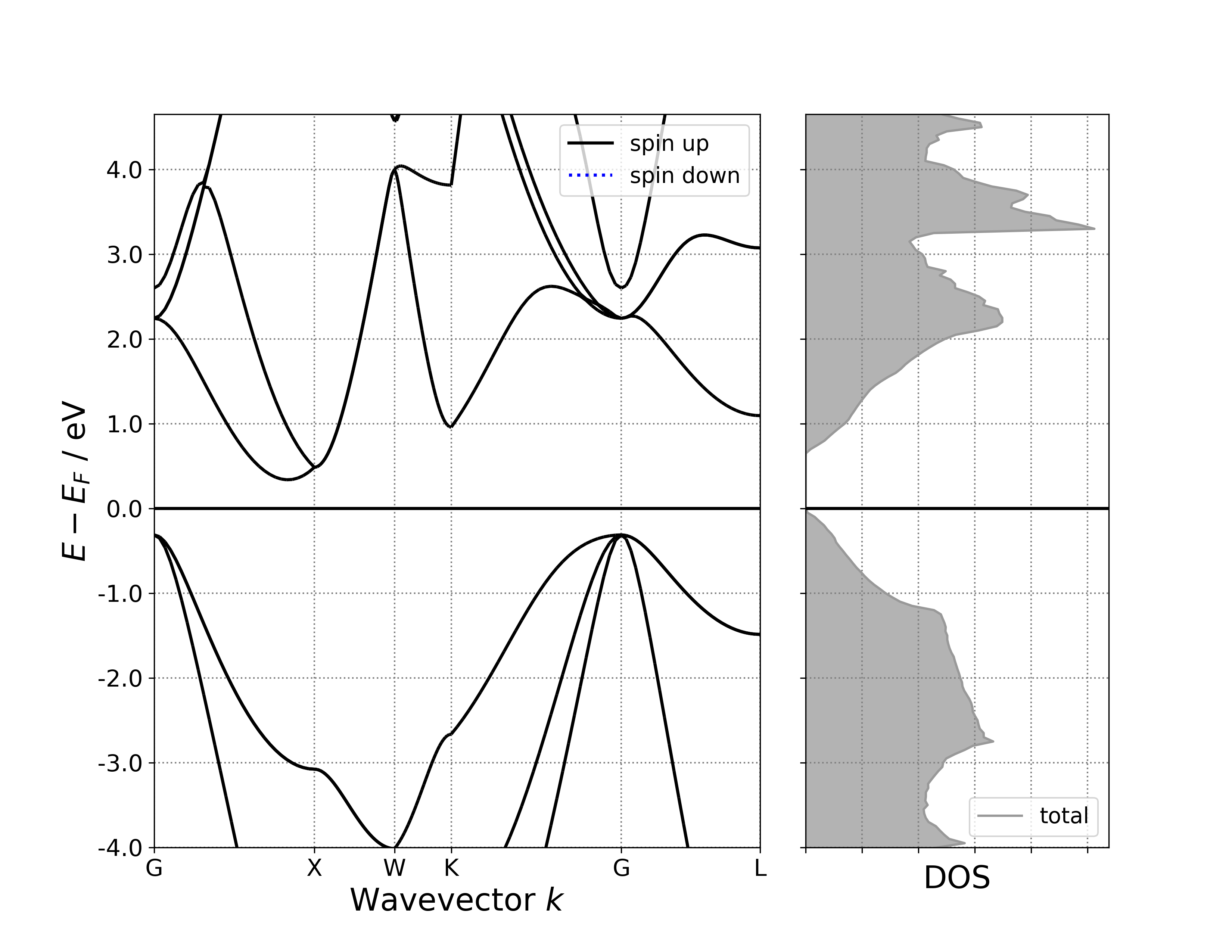
8.6 bandDos: Displaying Band Structure and Density of States Together
Using the Si system from the application tutorial as an example:
Display band structure and density of states in a single figure.
See 6bandDosplot.py:
 1# coding:utf-8
 2import os
 3
 4import numpy as np
 5from matplotlib.axes import Axes
 6from pymatgen.electronic_structure.plotter import BSDOSPlotter
 7
 8from dspawpy.io.read import get_band_data, get_dos_data
 9
10bandfile = "dspawpy_proj/dspawpy_tests/inputs/2.3/band.h5"  # Normal band data
11band_data = get_band_data(
12    band_dir=bandfile,
13    syst_dir=None,  # path to system.json file, required only when band_dir is a json file
14    efermi=None,  # Used for manually correcting the Fermi level
15)
16band_efermi = band_data.efermi
17dosfile = "dspawpy_proj/dspawpy_tests/inputs/2.5/dos.h5"  # Density of states data
18dos_data = get_dos_data(
19    dos_dir=dosfile,
20    return_dos=False,  # If False, always return a CompleteDos object (regardless of whether projection was enabled during calculation)
21)
22dos_efermi = dos_data.efermi
23bdp = BSDOSPlotter(
24    bs_projection=None,  # Band structure projection method, None means no projection
25    dos_projection=None,  # Projection method for density of states, None means no projection
26    vb_energy_range=4,  # Valence band energy range
27    cb_energy_range=4,  # Conduction band energy range
28    fixed_cb_energy=False,  # Whether to fix the conduction band energy range
29    egrid_interval=1,  # Energy grid interval
30    font="DejaVu Sans",  # Default is Times New Roman, change to DejaVu Sans to avoid warnings due to missing font on Linux
31    axis_fontsize=20,  # Axis font size
32    tick_fontsize=15,  # Tick label font size
33    legend_fontsize=14,  # Legend font size
34    bs_legend="best",  # Band structure legend position
35    dos_legend="best",  # Density of States legend position
36    rgb_legend=True,  # Use colored legend
37    fig_size=(11, 8.5),  # Figure size
38)
39if band_efermi != dos_efermi:
40    print(f"{band_efermi=:.4f} eV")
41    print(f"{dos_efermi=:.4f} eV")
42    d_efermi = band_efermi - dos_efermi
43
44    print(
45        "! Band and DOS Fermi levels are inconsistent, using DOS Fermi level as reference"
46    )
47    band_data.bands = {spin: v + d_efermi for spin, v in band_data.bands.items()}
48
49    # ! Band and DOS Fermi levels are inconsistent, using Band level as the reference
50    # dos_data.energies -= d_efermi
51
52axes_or_plt = bdp.get_plot(
53    bs=band_data, dos=dos_data
54)  # Pass band data  # Pass density of states data
55
56if isinstance(axes_or_plt, Axes):
57    fig = axes_or_plt.get_figure()  # version newer than v2023.8.10
58elif np.iterable(axes_or_plt):
59    fig = np.asarray(axes_or_plt).flatten()[0].get_figure()
60else:
61    fig = axes_or_plt.gcf()  # older version pymatgen
62
63filename = "dspawpy_proj/dspawpy_tests/outputs/us/6bandDos.png"  # Filename for the band structure - density of states plot output
64os.makedirs(os.path.dirname(os.path.abspath(filename)), exist_ok=True)
65fig.savefig(filename, dpi=300)
66print("==> Saved", filename)
Executing the code yields a band density of states plot similar to the following:
警告
If you are connecting to a remote server via SSH and running the above script, and you encounter QT-related error messages, it’s possible that the program you are using (such as MobaXterm) is incompatible with the QT libraries. You should either switch programs (e.g., VSCode or the system’s built-in terminal command line) or add the following code starting from the second line of your Python script:
import matplotlib
matplotlib.use('agg')
Display band structure and projected density of states on a single plot.
See 6bandPdosplot.py:
 1# coding:utf-8
 2import os
 3
 4import numpy as np
 5from matplotlib.axes import Axes
 6from pymatgen.electronic_structure.plotter import BSDOSPlotter
 7
 8from dspawpy.io.read import get_band_data, get_dos_data
 9
10bandfile = "dspawpy_proj/dspawpy_tests/inputs/2.4/band.h5"  # Normal band data
11band_data = get_band_data(
12    band_dir=bandfile,
13    syst_dir=None,  # path to system.json file, required only when band_dir is a json file
14    efermi=None,  # Used for manually correcting the Fermi level
15)
16band_efermi = band_data.efermi
17dosfile = (
18    "dspawpy_proj/dspawpy_tests/inputs/2.6/dos.h5"  # DOS data for projected states
19)
20dos_data = get_dos_data(
21    dos_dir=dosfile,
22    return_dos=False,  # If False, always return a CompleteDos object (regardless of whether projection was enabled during calculation)
23)
24dos_efermi = dos_data.efermi
25bdp = BSDOSPlotter(
26    bs_projection="elements",  # Projection method for band structure, None means no projection
27    dos_projection="elements",  # Project DOS onto elements
28    vb_energy_range=4,  # Valence band energy range
29    cb_energy_range=4,  # Conduction band energy range
30    fixed_cb_energy=False,  # Whether to fix the conduction band energy range
31    egrid_interval=1,  # Energy grid interval
32    font="DejaVu Sans",  # Default is Times New Roman, can be changed to DejaVu Sans to avoid warnings due to font not being installed on Linux
33    axis_fontsize=20,  # Axis font size
34    tick_fontsize=15,  # Tick label font size
35    legend_fontsize=14,  # Legend font size
36    bs_legend="best",  # Band structure legend position
37    dos_legend="best",  # Position of the projected density of states legend
38    rgb_legend=True,  # Use colored legend
39    fig_size=(11, 8.5),  # Figure size
40)
41if band_efermi != dos_efermi:
42    print(f"{band_efermi=:.4f} eV")
43    print(f"{dos_efermi=:.4f} eV")
44    d_efermi = band_efermi - dos_efermi
45
46    print(
47        "! Band and DOS Fermi levels are inconsistent, using DOS Fermi level as reference"
48    )
49    band_data.bands = {spin: v + d_efermi for spin, v in band_data.bands.items()}
50
51    # ! Band and DOS Fermi levels are inconsistent, using Band level as reference
52    # dos_data.energies -= d_efermi
53
54axes_or_plt = bdp.get_plot(
55    bs=band_data,
56    dos=dos_data,
57)  # Pass band structure data  # Pass projected density of states data
58
59if isinstance(axes_or_plt, Axes):
60    fig = axes_or_plt.get_figure()  # version newer than v2023.8.10
61elif np.iterable(axes_or_plt):
62    fig = np.asarray(axes_or_plt).flatten()[0].get_figure()
63else:
64    fig = axes_or_plt.gcf()  # older version pymatgen
65
66filename = "dspawpy_proj/dspawpy_tests/outputs/us/6bandPdos.png"  # filename for the band structure-projected density of states plot
67os.makedirs(os.path.dirname(os.path.abspath(filename)), exist_ok=True)
68fig.savefig(filename, dpi=300)
69print("==> Saved", filename)
Executing the code yields a band-decomposed density of states plot similar to the following:
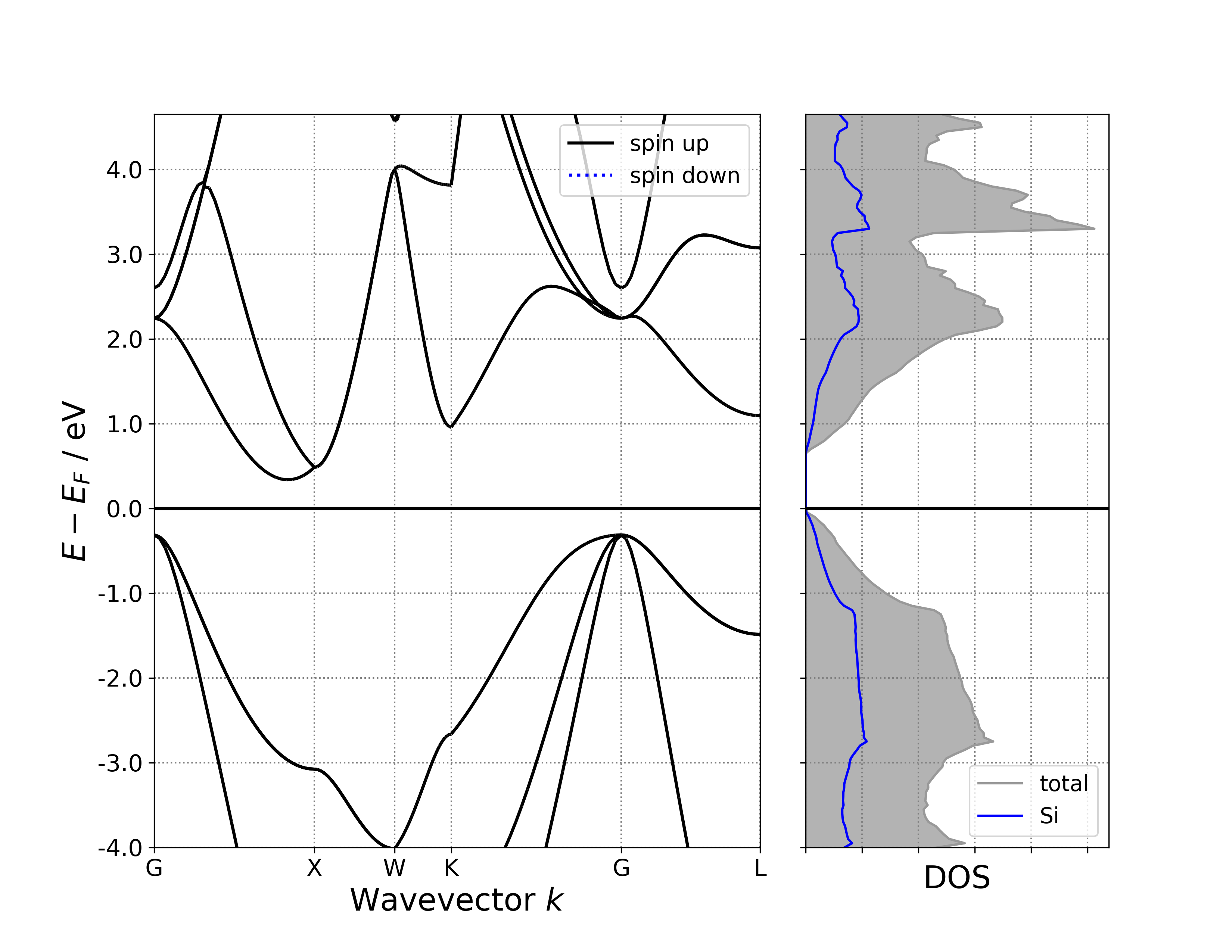
警告
Given projected band data, it will be projected along the element by default; given ordinary band data (or if the system contains more than 4 types of elements), it will not be projected and a warning will be output.
Given projected density of states (PDOS) data, projection along elements is also the default. You can switch to projection along orbitals, or no projection at all. For ordinary density of states (DOS) data and without disabling the DOS projection option BSDOSPlotter(dos_projection=None), the pymatgen plotting program will report an error, which is why a 6bandDosplot.py file was specifically prepared, as mentioned above.
警告
If you execute the above script by connecting to a remote server via SSH and encounter QT-related error messages, it’s likely due to incompatibility between the program you are using (e.g., MobaXterm) and the QT library. Either switch to a different program (such as VSCode or the system’s built-in terminal command line), or add the following code starting from the second line of your Python script:
import matplotlib
matplotlib.use('agg')
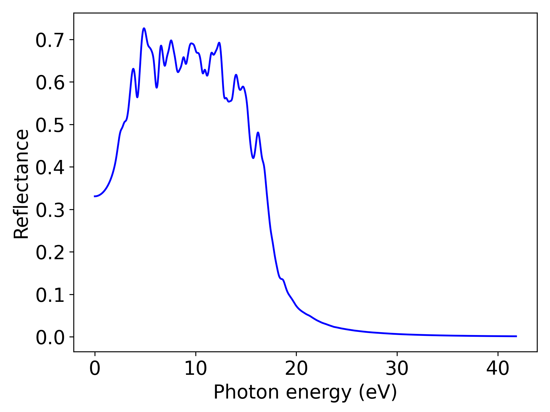
8.7 optical data processing
Using the scf.h5 file obtained from a quick start calculation of the optical properties of the Si system as an example (Note: the output file name is the same as the task, task = scf; io.optical = true can calculate optical properties):
Processing the reflectivity data, referring to 7optical.py:
 1# coding:utf-8
 2from dspawpy.plot import plot_optical
 3
 4plot_optical(
 5    datafile="dspawpy_proj/dspawpy_tests/inputs/2.12/scf.h5",
 6    keys=["ExtinctionCoefficient", "Reflectance"],
 7    axes=["X"],  # ["X", "Y", "Z", "XY", "YZ", "ZX"]
 8    prefix="dspawpy_proj/dspawpy_tests/outputs/optical",  # Where to save, if empty, it means the current folder
 9    save=True,  # Whether to save the image with the tool's name, if False, please refer to the script below to save manually
10)
11
12# The above function will plot and save the images of ExtinctionCoefficient and Reflectance separately
13# To plot multiple properties on the same figure, uncomment the following code and set the save parameter above to False
14
15# import os
16# import matplotlib.pyplot as plt
17#
18# plt.tick_params(labelsize=16)
19# plt.tight_layout()
20# filename = "outputs/us/7optical.png"  # Filename for the output optical properties plot
21# os.makedirs(os.path.dirname(os.path.abspath(filename)), exist_ok=True)
22# plt.savefig(filename, dpi=300)
备注
Reflectance is an optical property, and users can modify this keyword to “AbsorptionCoefficient”, “ExtinctionCoefficient”, or “RefractiveIndex” based on their needs, corresponding to the absorption coefficient, extinction coefficient, and refractive index, respectively.
Executing the code will generate a curve showing the reflectance as a function of energy, similar to the following:
警告
If you execute the above script by connecting to a remote server via SSH and encounter QT-related error messages, it is likely that the program you are using (such as MobaXterm, etc.) is incompatible with the QT libraries. You can either switch to another program (such as VSCode or the system’s built-in terminal command line) or add the following code to your Python script, starting from the second line:
import matplotlib
matplotlib.use('agg')
8.8 neb data processing
Let’s start with a quick introduction using the H diffusion on Pt(100) surface example:
Generating intermediate configurations for input files
See
8neb_interpolate_structures.py:1# coding:utf-8 2from dspawpy.diffusion.neb import NEB, write_neb_structures 3from dspawpy.diffusion.nebtools import write_json_chain 4from dspawpy.io.structure import read 5 6# Read initial configuration 7init_struct = read("dspawpy_proj/dspawpy_tests/inputs/2.15/00/structure00.as")[0] 8# Read final state configuration 9final_struct = read("dspawpy_proj/dspawpy_tests/inputs/2.15/04/structure04.as")[0] 10 11neb = NEB( 12 initial_structure=init_struct, # Initial structure 13 final_structure=final_struct, # Final state configuration 14 nimages=8, # Total of 8 configurations, including initial and final states 15) 16structures = neb.linear_interpolate() # Linear interpolation 17# structures = neb.idpp_interpolate() # IDPP interpolation 18 19# Save as structure file to dest path 20write_neb_structures( 21 structures=structures, # Insert interpolated structure chains 22 coords_are_cartesian=True, # Whether to save in Cartesian coordinates 23 fmt="as", # Save format, supported formats: 'json', 'as', 'hzw', 'pdb', 'xyz', 'dump' 24 path="dspawpy_proj/dspawpy_tests/outputs/us/8neb_interpolate_structures", # Save path 25 prefix="structure", # File name prefix 26) 27 28# Preview initial structure chain 29write_json_chain( 30 preview=True, # whether to enable preview mode 31 directory="dspawpy_proj/dspawpy_tests/outputs/us/8neb_interpolate_structures", # Directory for NEB calculations 32 step=-1, # Default to saving the structure chain of the last ion step (latest) 33 dst="dspawpy_proj/dspawpy_tests/outputs/us/8neb", # Save path 34) 35# write_xyz_chain(preview=True, # Whether to run in preview mode 36# directory="dspawpy_proj/dspawpy_tests/outputs/us/8neb_interpolate_structures", # NEB calculation directory 37# step=-1, # Default to saving the structure chain of the last ionic step (latest) 38# dst='dspawpy_proj/dspawpy_tests/outputs/us/8neb' # save path 39# )
备注
Users can modify the number of interpolated points as needed. Setting it to 8 will generate a folder containing 8 structure files, with 6 intermediate configurations.
neb.linear_interpolateis a linear interpolation method. Thepbcparameter, when set toTrue, will lock the search for the shortest diffusion path. It defaults toFalseto increase user control, becauseFor example, if the initial fractional coordinate of an atom is 0.2 and the final state is 0.8. When pbc = True, the diffusion path will be forced to be 0.2 -> -0.2. When pbc = False, the user can make the program perform interpolation along the diffusion path 0.2 -> 0.8; if the shortest path is desired, manually change 0.8 to -0.2, thereby ensuring the program completes the initial guess of interpolation according to the user’s intent.
Plotting the energy barrier diagram
neb.iniFin = true/false
When neb.iniFin = true/false, you can use the path from the NEB calculation for barrier analysis (ensure that the initial and final state calculation files are in the NEB calculation path):
Refer to
8neb_barrier_CubicSpline.py:1# coding:utf-8 2from dspawpy.diffusion.nebtools import plot_barrier 3 4directory_of_neb_task = ( 5 "dspawpy_proj/dspawpy_tests/inputs/2.15" # <-- Please modify to the actual NEB path 6) 7 8# Plotting the energy barrier using CubicSpline interpolation 9plot_barrier( 10 directory=directory_of_neb_task, # path of the neb task 11 method="CubicSpline", # Cubic spline interpolation 12 figname="dspawpy_proj/dspawpy_tests/outputs/us/8neb_barrier_CubicSpline.png", # Output filename for the energy barrier plot 13 show=False, # Whether to display the energy barrier plot 14)
备注
After running the above script, you can obtain a barrier curve similar to the following, with cubic spline interpolation:
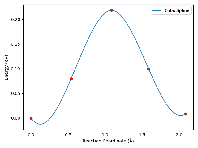
For this specific example, the curve will exhibit an undesirable “dip” after cubic spline interpolation, which is inherent to the characteristics of the cubic spline interpolation algorithm.
dspawpy internally calls scipy’s interpolation algorithms. Taking the cubic spline interpolation algorithm as an example in the script above, it is defined in the scipy documentation as:
class scipy.interpolate.CubicSpline(x, y, axis=0, bc_type='not-a-knot', extrapolate=None)
The keyword arguments include axis, bc_type, and extrapolate, whose specific meanings can be found in scipy.interpolate.CubicSpline. We can specify the corresponding keyword arguments (axis, bc_type, extrapolate) in the plot_barrier function and pass them to the scipy.interpolate.CubicSpline class for processing.
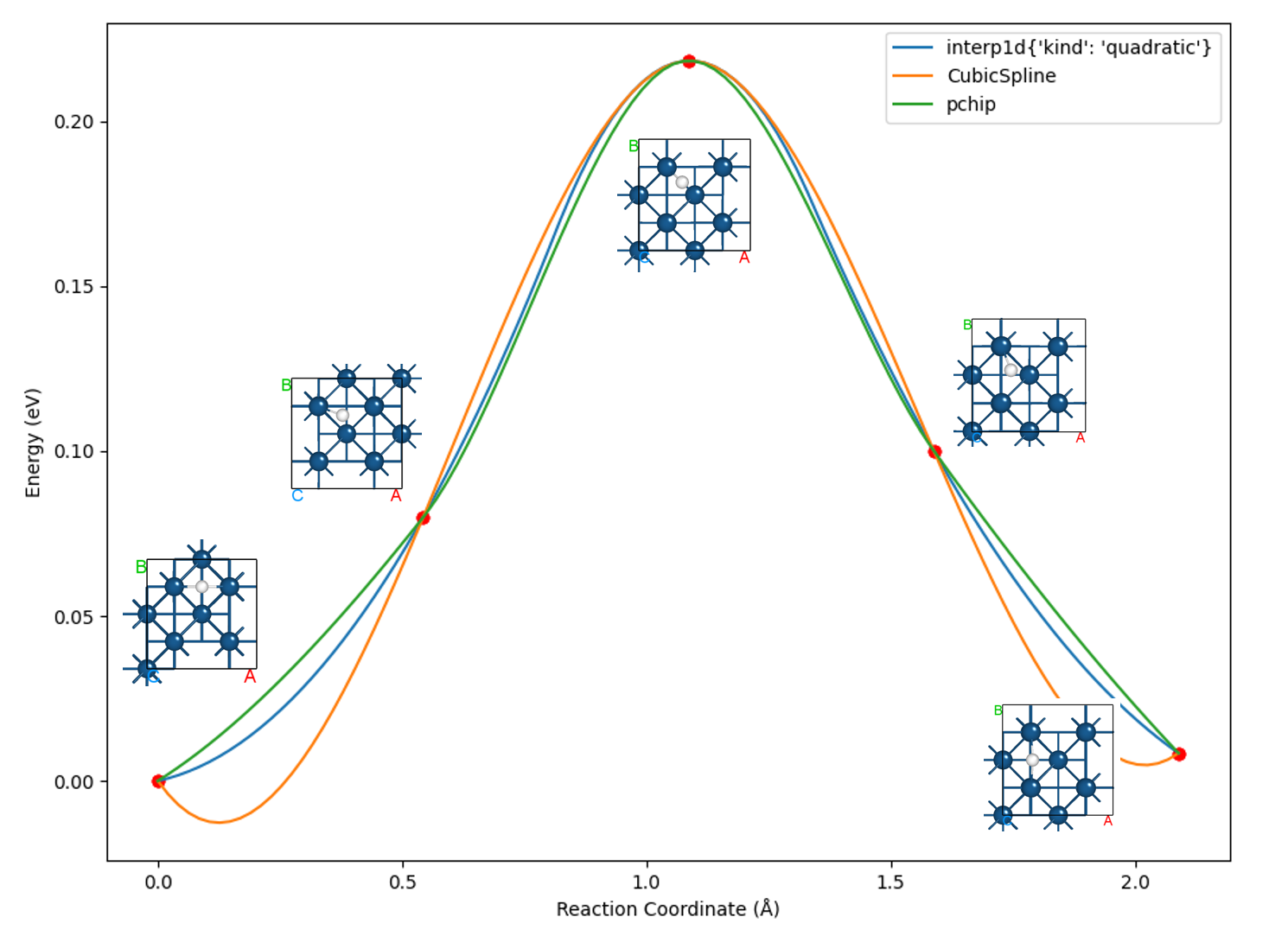
Here we use the script 8neb_barrier.py to compare the curves plotted by interpolating with three algorithms:
 1# coding:utf-8
 2import os
 3
 4import matplotlib.pyplot as plt
 5
 6from dspawpy.diffusion.nebtools import plot_barrier
 7
 8# Compare the differences in energy barrier curves drawn by different interpolation methods, where show should be set to False
 9# 1. interp1d
10plot_barrier(
11    directory="dspawpy_proj/dspawpy_tests/inputs/2.15",  # path for NEB calculation
12    ri=None,  # Reaction coordinate between the initial structure and the second structure, required when the NEB task only calculated intermediate structures
13    rf=None,  # Reaction coordinate between the last configuration and the second-to-last configuration, when the NEB task only calculated intermediate configurations
14    ei=None,  # Energy of the initial configuration, required when the NEB task only calculated intermediate configurations
15    ef=None,  # Energy of the final configuration, required when the NEB task only calculated intermediate configurations
16    method="interp1d",  # Interpolation method
17    figname=None,  # Name of the output energy barrier plot file
18    show=False,  # Whether to display the energy barrier plot
19    kind="quadratic",  # Parameter of the interpolation method
20)
21# 2. CubicSpline
22plot_barrier(
23    directory="dspawpy_proj/dspawpy_tests/inputs/2.15",
24    method="CubicSpline",
25    figname=None,
26    show=False,
27)
28# 3. pchip
29plot_barrier(
30    directory="dspawpy_proj/dspawpy_tests/inputs/2.15",
31    method="pchip",
32    figname=None,
33    show=False,
34)
35
36filename = "dspawpy_proj/dspawpy_tests/outputs/us/8neb_barrier_comparison.png"  # Filename for the energy barrier plot output
37os.makedirs(os.path.dirname(os.path.abspath(filename)), exist_ok=True)
38plt.savefig(filename, dpi=300)
39# plt.show()
备注
Choosing the appropriate interpolation algorithm is crucial for optimizing the final curve presentation.
In most cases, selecting the pchip (piecewise cubic Hermite interpolating polynomial) monotonic cubic spline interpolation algorithm will achieve good results, and it is also the default interpolation algorithm called.
neb.iniFin = true
When neb.iniFin = true is set, reading the neb.h5/neb.json files generated by the NEB calculation allows for a quick barrier analysis:
See
8neb_barrier_CubicSpline.py:1# coding:utf-8 2from dspawpy.diffusion.nebtools import plot_barrier 3 4# Plot energy barrier using CubicSpline interpolation 5plot_barrier( 6 datafile="dspawpy_proj/dspawpy_tests/inputs/2.15/neb.h5", # Path to neb.h5 7 method="CubicSpline", # Cubic spline interpolation 8 figname="dspawpy_proj/dspawpy_tests/outputs/us/8neb_barrier_.png", # Output file name for the energy barrier plot 9 show=False, # Whether to display the energy barrier plot 10)
Processing the resulting barrier diagram is consistent with the previously read path.
备注
The energy stored in neb.h5 and neb.json files is TotalEnergy. If you need an accurate barrier value, it is recommended to process it by reading the NEB calculation path (taking TotalEnergy0).
警告
If you are connecting to a remote server via SSH to execute the script above and encounter QT-related error messages, it’s possible that the program you are using (e.g., MobaXterm) is incompatible with the QT libraries. Either switch to a different program (such as VSCode or the system’s built-in terminal command line), or add the following code starting on the second line of your Python script:
import matplotlib
matplotlib.use('agg')
Processing Data for Transition State Calculations
After NEB calculations, it is generally necessary to plot the energy barrier diagram and check the forces on each interpolated structure to ensure they are below a specified threshold. If the results are abnormal, the force and energy changes of each interpolated structure during the structure optimization process should also be checked to determine if they have truly “converged.” These operations require at least three cycles. To simplify the process, we provide an all-in-one summary function summary:
Refer to
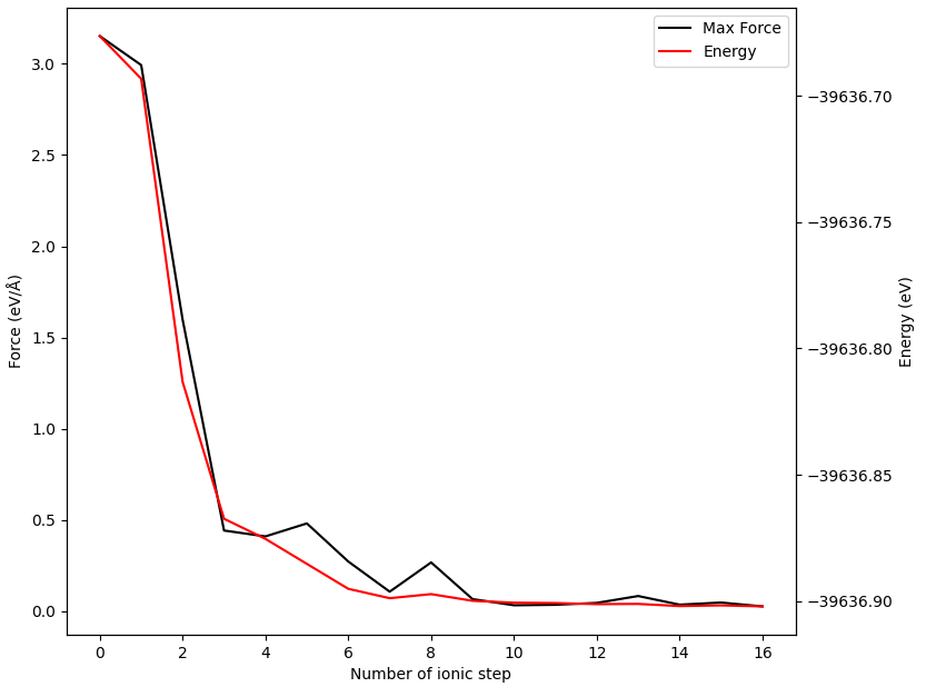
8neb_check_results.py:1# coding:utf-8 2from dspawpy.diffusion.nebtools import summary 3 4# Import the neb calculation directory, a complete folder after neb calculation needs to be provided 5summary( 6 directory="dspawpy_proj/dspawpy_tests/inputs/2.15", 7 show_converge=False, # Whether to display the convergence plots of energy and force 8 outdir="dspawpy_proj/dspawpy_tests/outputs/us/8neb", # Path to save convergence plots of energy and forces 9 figname="dspawpy_proj/dspawpy_tests/outputs/us/8neb/neb_barrier_summary.png", # Path to save the energy barrier plot 10) 11# Additional keyword arguments can be set for plotting the barrier diagram, such as: 12# summary(directory='dspawpy_proj/dspawpy_tests/inputs/2.15', method='CubicSpline') # Change to CubicSpline for spline interpolation
备注
This script will print the energies and forces of each structure in a table, plot the energy barrier, and also plot the convergence of energy and forces for intermediate structures.
If
neb.iniFin = false, the user must copy the results file of the self-consistent calculation, either scf.h5 or system.json, to the corresponding initial and final state subfolders. Otherwise, the program cannot read the energy and force information of the initial and final states and will exit with an error.By default, the energy barrier plot is stored in the parent directory of the NEB calculation, and the energy and force convergence plots for each intermediate structure are stored in the respective subfolders.
Executing the code will generate a table similar to the following, displaying the energy and force information for each NEB configuration:
Image
Force (eV/Å)
Reaction coordinate (Å)
Energy (eV)
Delta energy (eV)
00
0.1803
0.0000
-39637.0984
0.0000
01
0.0263
0.5428
-39637.0186
0.0798
02
0.0248
1.0868
-39636.8801
0.2183
03
0.2344
1.5884
-39636.9984
0.1000
04
0.0141
2.0892
-39637.0900
0.0084
In addition to the energy barrier diagram, you can also obtain the energy and force convergence curves for each intermediate configuration (taking configuration 02 as an example).
警告
If you execute the above script by connecting to a remote server via SSH and encounter QT-related error messages, it might be due to incompatibility between the program you are using (such as MobaXterm) and the QT library. Either switch to another program (such as VSCode or the system’s built-in terminal command line), or add the following code starting from the second line of your Python script:
import matplotlib
matplotlib.use('agg')
Observing the NEB Chain
Here, the NEB chain refers to the geometric relationship between the interpolated structures (structure00.as, structure01.as, …), rather than the changes of a single structure during the optimization process.
NEB calculations are computationally expensive, and observing the NEB chain helps to judge the convergence speed of the NEB calculation. Furthermore, after generating intermediate structures via interpolation, previewing the NEB chain is often necessary. These needs can be met using the
8neb_visualize.pyscript:
 1# coding:utf-8
 2from dspawpy.diffusion.nebtools import write_json_chain, write_xyz_chain
 3
 4# Convert the configuration chain under the NEB calculation path to a JSON format file
 5write_json_chain(
 6    preview=False,  # If the NEB calculation is already completed, preview mode is not required
 7    directory="dspawpy_proj/dspawpy_tests/inputs/2.15",  # NEB calculation directory
 8    step=-1,  # Default to saving the configuration chain of the last ion step (latest)
 9    dst="dspawpy_proj/dspawpy_tests/outputs/us/8neb",  # Save path
10    ignorels=False,  # Set to True to ignore latestStructureXX.as files
11)
12
13# Convert the configuration chain in the NEB calculation path to xyz format files
14write_xyz_chain(
15    preview=False,  # If the NEB calculation is already completed, preview mode is not required
16    directory="dspawpy_proj/dspawpy_tests/inputs/2.15",  # NEB calculation directory
17    step=-1,  # Default to saving the configuration chain of the last ionic step (latest)
18    dst="dspawpy_proj/dspawpy_tests/outputs/us/8neb",  # Save path
19    ignorels=False,  # Set to True to ignore latestStructureXX.as files
20)
备注
After this script generates the neb_movie*.json files, you can view them by opening the json file via
Device Studio–>Simulator–>DS-PAW–>Analysis Plot.The directory parameter specifies the main path of the NEB calculation; the complete folder after the NEB calculation is finished must be provided.
This script supports processing ongoing (i.e., incomplete) NEB calculation files, allowing users to monitor the trajectory in real time.
The xyz file can be opened and viewed using OVITO software: Open the visualization interface via
Device Studio–>Simulator–>OVITO, and then drag and drop the xyz file.Structure information reading priority: latestStructureXX.as > h5 > json; When ignorels is set to True, it first attempts to read data from h5, and if it fails, it reads from json.
Calculate the inter-configuration distance
Refer to this script:
8calc_dist.py:1# coding:utf-8 2from dspawpy.diffusion.nebtools import get_distance 3from dspawpy.io.structure import read 4 5# Please modify the paths of structure01.as and structure02.as structure files according to the actual situation 6# First read the fractional coordinates, element list, and cell information of the two configurations 7s1 = read("dspawpy_proj/dspawpy_tests/inputs/2.15/01/structure01.as")[0] 8s2 = read("dspawpy_proj/dspawpy_tests/inputs/2.15/02/structure02.as")[0] 9# Calculate the distance between the two configurations, note that this function only accepts fractional coordinates 10dist = get_distance( 11 spo1=s1.frac_coords, 12 spo2=s2.frac_coords, 13 lat1=s1.lattice.matrix, 14 lat2=s2.lattice.matrix, 15) 16print("The distance between the two configurations is:", dist, "Angstrom")
Continued calculation with neb
To restart a NEB calculation, refer to
8neb_restart.py:1# coding:utf-8 2import os 3from shutil import copytree, rmtree 4 5from dspawpy.diffusion.nebtools import restart 6 7if os.path.isdir("dspawpy_proj/dspawpy_tests/outputs/us/neb4bk"): 8 rmtree("dspawpy_proj/dspawpy_tests/outputs/us/neb4bk") 9 10copytree( 11 "dspawpy_proj/dspawpy_tests/inputs/2.15", 12 "dspawpy_proj/dspawpy_tests/outputs/us/neb4bk", 13) 14restart( 15 directory="dspawpy_proj/dspawpy_tests/outputs/us/neb4bk", # NEB task path 16 output="dspawpy_proj/dspawpy_tests/outputs/us/8neb_restart", # Backup destination 17)
See Continued calculation with neb for details.
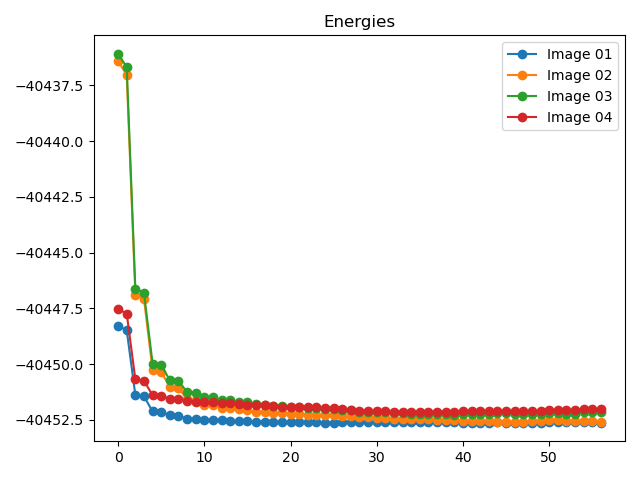
Energy and maximum atomic force variation trend during NEB calculation
To view plots showing the energy and maximum atomic force trends during the NEB calculation, refer to
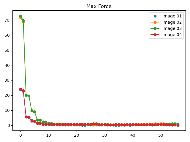
8neb_energy_force_curves.py:1# coding:utf-8 2from dspawpy.diffusion.nebtools import monitor_force_energy 3 4# Specify the path to the NEB calculation folder; after running, Energies.png and MaxForce.png images will be generated in the specified directory 5unfinished_neb_folder = "dspawpy_proj/dspawpy_tests/inputs/supplement/neb_unfinished" 6monitor_force_energy( 7 directory=unfinished_neb_folder, 8 outdir="imgs", # Output image path 9)
Generates energy and force change trend charts:
8.9 Phonon Data Processing
Using the example of a phonon band structure and density of states calculation for MgO, using phonon.h5:
If phonopy is not installed, running the following script will result in the message no module named 'phonopy', but this does not affect the program’s normal operation.
Phonon band data processing
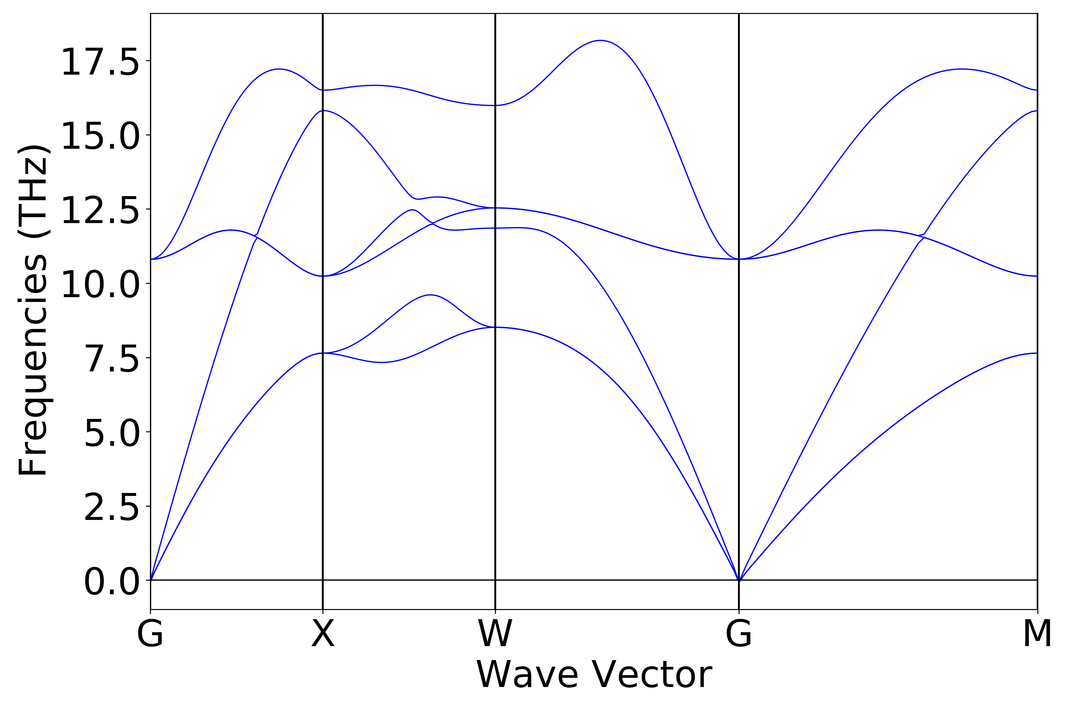
Refer to
9phonon_bandplot.py:
 1# coding:utf-8
 2import os
 3
 4from pymatgen.phonon.plotter import PhononBSPlotter
 5
 6from dspawpy.io.read import get_phonon_band_data
 7
 8band_data = get_phonon_band_data(
 9    "dspawpy_proj/dspawpy_tests/inputs/2.16.1/phonon.h5",
10)  # Read phonon band structure
11bsp = PhononBSPlotter(band_data)
12axes_or_plt = bsp.get_plot(ylim=None, units="thz")  # Y-axis range # Units
13import matplotlib.pyplot as plt  # noqa: E402
14
15if isinstance(axes_or_plt, plt.Axes):
16    fig = axes_or_plt.get_figure()  # version newer than v2023.8.10
17elif isinstance(axes_or_plt, tuple):
18    fig = axes_or_plt[0].get_figure()
19else:
20    fig = axes_or_plt.gcf()  # older version pymatgen
21
22filename = "dspawpy_proj/dspawpy_tests/outputs/us/9phonon_bandplot.png"  # File name for the output phonon band plot
23os.makedirs(os.path.dirname(os.path.abspath(filename)), exist_ok=True)
24fig.savefig(filename, dpi=300)
Executing the code yields a phonon band structure curve similar to the following:
警告
If you encounter QT-related error messages when executing the above script via SSH connection to a remote server, it’s likely due to incompatibility between the program used (e.g., MobaXterm) and the QT library. Either change the program (e.g., VSCode or the system’s built-in terminal command line), or add the following code to your Python script starting from the second line:
import matplotlib
matplotlib.use('agg')
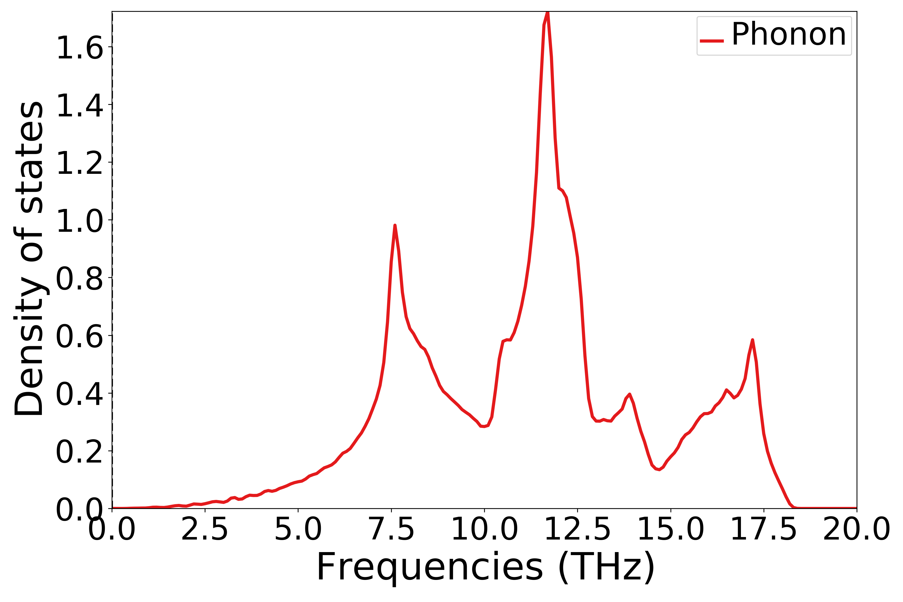
Phonon Density of States Data Processing
Refer to
9phonon_dosplot.py:1# coding:utf-8 2import os 3 4from pymatgen.phonon.plotter import PhononDosPlotter 5 6from dspawpy.io.read import get_phonon_dos_data 7 8dos = get_phonon_dos_data("dspawpy_proj/dspawpy_tests/inputs/2.16.1/phonon.h5") 9dp = PhononDosPlotter( 10 stack=False, # True indicates drawing an area plot 11 sigma=None, # Gaussian blur parameter 12) 13dp.add_dos( 14 label="Phonon", dos=dos 15) # Legend # The phonon density of states to be plotted 16axes_or_plt = dp.get_plot( 17 xlim=[0, 20], # x-axis range 18 ylim=None, # y-axis range 19 units="THz", # Unit 20) 21import matplotlib.pyplot as plt # noqa: E402 22 23if isinstance(axes_or_plt, plt.Axes): 24 fig = axes_or_plt.get_figure() # version newer than v2023.8.10 25elif isinstance(axes_or_plt, tuple): 26 fig = axes_or_plt[0].get_figure() 27else: 28 fig = axes_or_plt.gcf() # older version pymatgen 29 30filename = " dspawpy_proj/dspawpy_tests/outputs/us/9phonon_dosplot.png" # Energy barrier plot output filename 31os.makedirs(os.path.dirname(os.path.abspath(filename)), exist_ok=True) 32fig.savefig(filename, dpi=300)
Executing the code yields a phonon density of states curve similar to the following:
警告
If you execute the script above by SSH connection to a remote server and encounter QT-related error messages, it’s possible that the program you are using (such as MobaXterm) is incompatible with the QT library. Either change the program (e.g., VSCode or the system’s built-in terminal command line), or add the following code starting from the second line of your Python script:
import matplotlib
matplotlib.use('agg')
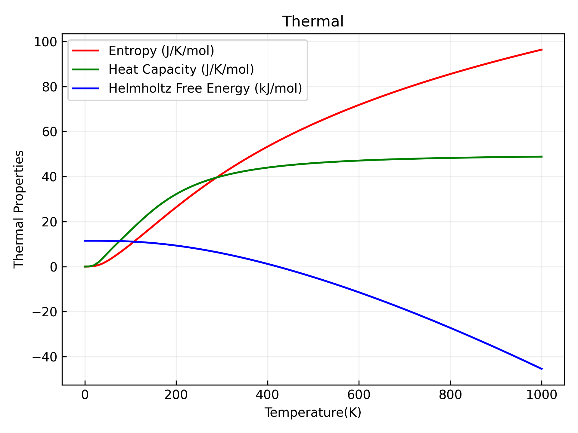
Phonon Thermodynamic Data Processing
Refer to 9phonon_thermal.py:
1# coding:utf-8
2from dspawpy.plot import plot_phonon_thermal
3
4plot_phonon_thermal(
5    datafile="dspawpy_proj/dspawpy_tests/inputs/2.26/phonon.h5",  # phonon.h5 data file path
6    figname="dspawpy_proj/dspawpy_tests/outputs/us/9phonon.png",  # Output phonon thermodynamics figure filename
7    show=False,  # Whether to display the image
8)
Executing the code yields phonon thermodynamic curves similar to the following:
警告
If you execute the above script by connecting to a remote server via SSH and encounter QT-related error messages, it’s likely that the program you are using (e.g., MobaXterm) is incompatible with the QT libraries. You can either switch programs (e.g., VSCode or the system’s built-in terminal) or add the following code starting from the second line of your Python script:
import matplotlib
matplotlib.use('agg')
8.10 aimd molecular dynamics simulation data processing
For a quick start, take the molecular dynamics simulation data of the \(H_{2}O\) molecular system, for example, the aimd.h5 file:
Convert the trajectory file format to .xyz or .dump.
Read data from the HDF5 file output by AIMD and generate trajectory files.
The generated .xyz or .dump files can be dragged and dropped into OVITO for visualization. You can open the OVITO visualization interface through Device Studio –> Simulator –> OVITO, and then drag and drop the .xyz or .dump files into OVITO.
See 10write_aimd_traj.py:
 1# coding:utf-8
 2from dspawpy.io.structure import convert
 3
 4convert(
 5    infile="dspawpy_proj/dspawpy_tests/inputs/2.18/aimd.h5",  # Structure to be converted, if in the current path, only the filename can be written
 6    si=None,  # Filter the configuration number, if not specified, read all by default
 7    ele=None,  # Filter element symbol, default reads atomic information for all elements
 8    ai=None,  # Filter atomic indices (starting from 1), default to read all atomic information
 9    outfile="dspawpy_proj/dspawpy_tests/outputs/us/10aimdTraj.xyz",  # Can also generate .dump files (lower precision), currently only supports orthogonal unit cells
10)
Executing the code will generate trajectory files in .xyz and .dump formats, which can be opened with OVITO. For more details on structure file conversion, refer to structure structure conversion
备注
OVITO and dspawpy do not support saving systems with non-orthogonal unit cells as dump files.
Changes in energy, temperature, etc. curves during the dynamics process.
Refer to
10check_aimd_conv.py:1# coding:utf-8 2from dspawpy.plot import plot_aimd 3 4plot_aimd( 5 datafile="dspawpy_proj/dspawpy_tests/inputs/2.18/aimd.h5", # Data file path 6 show=False, # Whether to pop up the image window 7 figname="dspawpy_proj/dspawpy_tests/outputs/us/10aimd.png", # Output image file name 8 flags_str="1 2 3 4 5", # Select data types 9) 10# The meaning of flags_str is as follows 11# 1. Kinetic energy 12# 2. Total Energy 13# 3. Pressure 14# 4. Temperature 15# 5. Volume
Executing the code will generate the following combined graph:
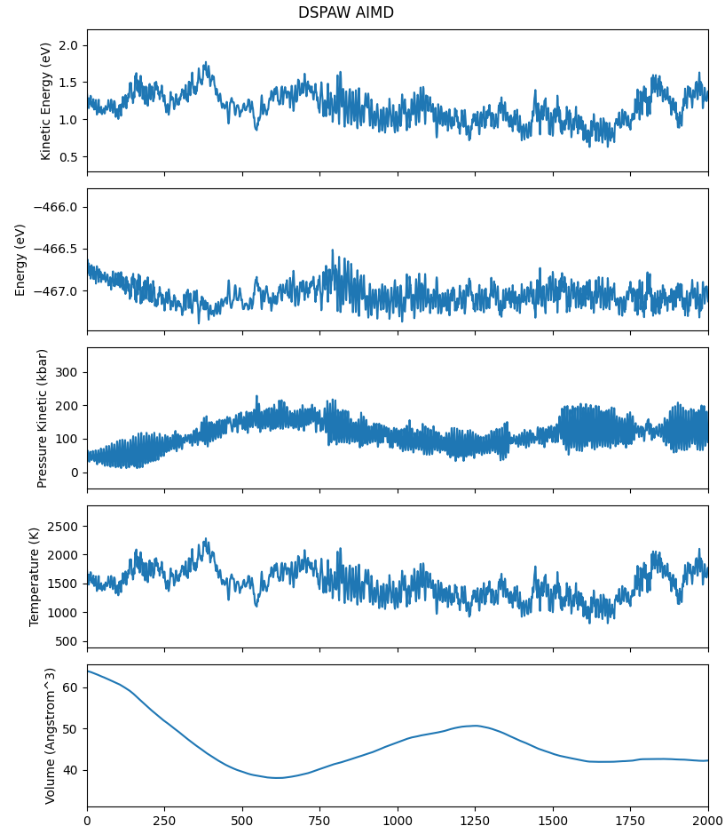
警告
If you execute the above script by SSH connection to a remote server and encounter QT-related error messages, it’s possible that the program you are using (such as MobaXterm) is incompatible with the QT libraries. You can either switch programs (for example, VSCode or the system’s built-in terminal command line), or add the following code starting from the second line of the Python script:
import matplotlib
matplotlib.use('agg')
Mean Squared Displacement (MSD) Analysis
See
10aimd_msd.py:1# coding:utf-8 2from dspawpy.analysis.aimdtools import get_lagtime_msd, plot_msd 3 4# If AIMD is not completed in one go, you can assign multiple h5 file paths to the datafile parameter in a list form 5lagtime, msd = get_lagtime_msd( 6 datafile="dspawpy_proj/dspawpy_tests/inputs/2.18/aimd.h5", # Data file path 7 select="all", # Default selects all atoms 8 msd_type="xyz", # Default to calculate MSD in the xyz directions 9 timestep=None, # Default reads the timestep from the datafile 10) 11# Plot the graph using the obtained data and save it 12plot_msd( 13 lagtime, # X-axis coordinate 14 msd, # vertical axis 15 xlim=None, # Set the display range of the x-axis 16 ylim=None, # Set the display range of the y-axis 17 figname="dspawpy_proj/dspawpy_tests/outputs/us/10MSD.png", # Output image filename 18 show=False, # Whether to pop up the image window 19 ax=None, # Optional subplot specification 20)
Executing the code will generate an image similar to the following:
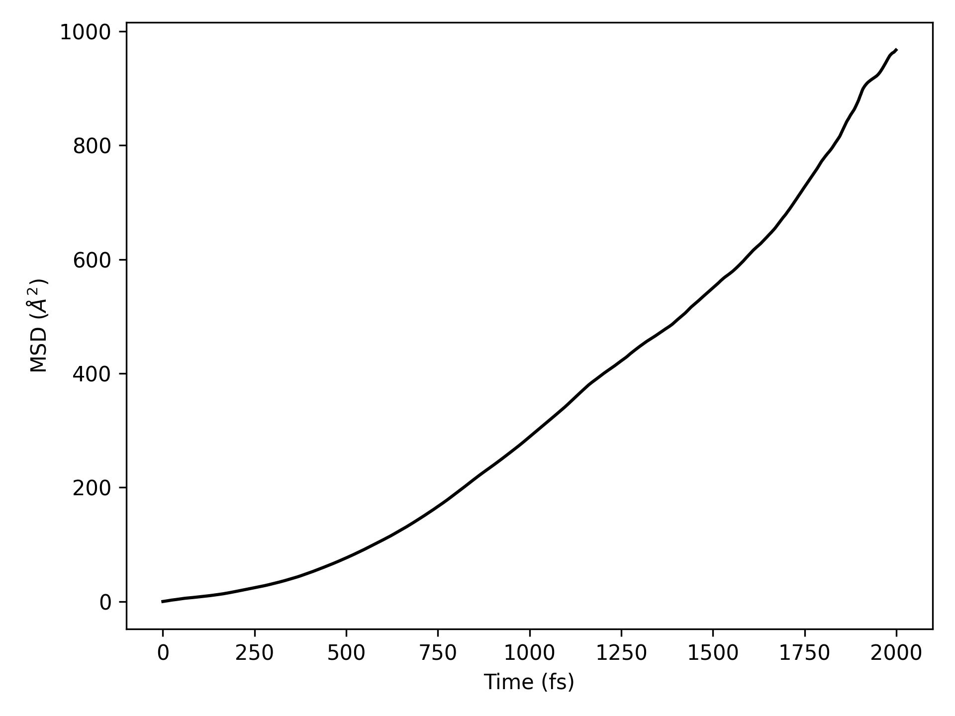
警告
If you execute the above script by SSH connection to a remote server and encounter QT-related error messages, it might be due to incompatibility between the program you’re using (like MobaXterm, etc.) and the QT libraries. Either switch to a different program (such as VSCode or the system’s built-in terminal), or add the following code starting from the second line of the Python script:
import matplotlib
matplotlib.use('agg')
Root Mean Square Deviation (RMSD) Analysis
See
10aimd_rmsd.py:1# coding:utf-8 2from dspawpy.analysis.aimdtools import get_lagtime_rmsd, plot_rmsd 3 4# If AIMD is not completed in a single run, you can assign multiple paths of h5 files in list form to the datafile parameter 5lagtime, rmsd = get_lagtime_rmsd( 6 datafile="dspawpy_proj/dspawpy_tests/inputs/2.18/aimd.h5", 7 timestep=None, # Data file path # Default reads the time step from the datafile 8) 9plot_rmsd( 10 lagtime, # Horizontal coordinate 11 rmsd, # vertical coordinate 12 xlim=None, # Set the display range of the x-axis 13 ylim=None, # Set the display range of the y-axis 14 figname="dspawpy_proj/dspawpy_tests/outputs/us/10RMSD.png", # Output image filename 15 show=False, # Whether to pop up the image window 16 ax=None, # Optional subplot specification 17)
Executing the code will generate an image similar to the following:
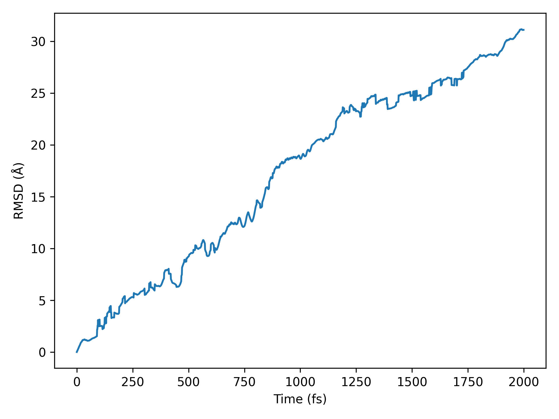
警告
If you execute the above script by connecting to a remote server via SSH, and QT-related error messages appear, it may be due to incompatibility between the program used (e.g., MobaXterm) and the QT libraries. Either change the program (such as VSCode or the system’s built-in terminal command line), or add the following code starting from the second line of your Python script:
import matplotlib
matplotlib.use('agg')
Analysis of Atomic Pair Distribution Functions or Radial Distribution Functions (RDFs)
See
10aimd_rdf.py:1# coding:utf-8 2from dspawpy.analysis.aimdtools import get_rs_rdfs, plot_rdf 3 4# If AIMD is not completed in one go, you can assign multiple h5 file paths to the datafile parameter in the form of a list. 5rs, rdfs = get_rs_rdfs( 6 datafile="dspawpy_proj/dspawpy_tests/inputs/2.18/aimd.h5", # Data file path 7 ele1="H", # Central element 8 ele2="O", # Target element 9 rmin=0.0, # Minimum radius 10 rmax=10.0, # Maximum radius 11 ngrid=1000, # Number of grid points 12 sigma=0.1, # sigma value 13) 14plot_rdf( 15 rs, # x-axis values 16 rdfs, # Vertical coordinate 17 "H", # Central element 18 "O", # Object element 19 figname="dspawpy_proj/dspawpy_tests/outputs/us/10RDF.png", # Image save path 20 show=False, # Whether to pop up the image window 21 ax=None, # Subplot can be specified 22)
Executing the code will generate an image similar to the following:
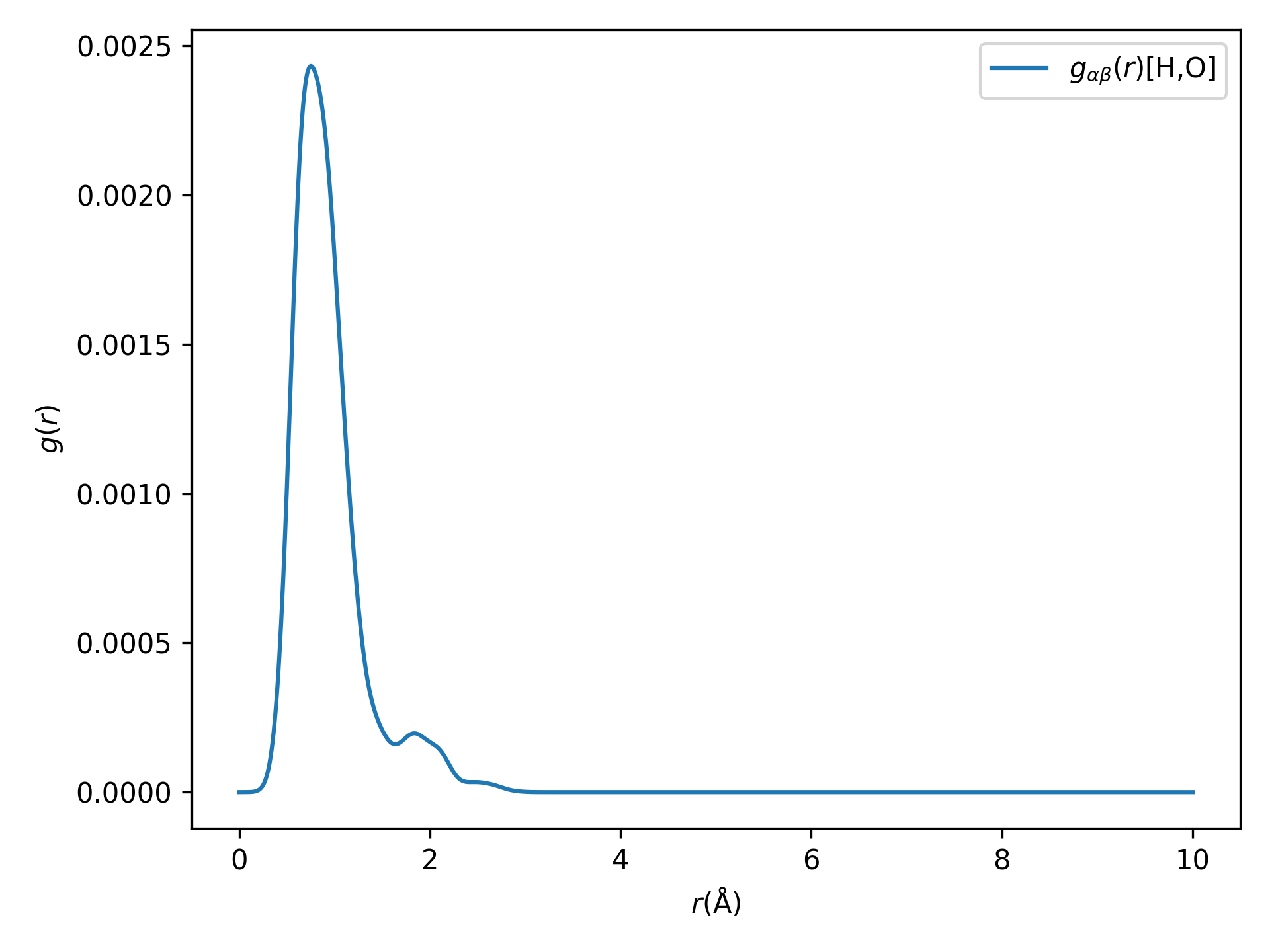
The statistical calculations involved in this section are complex; please refer to the function API for more details.
警告
If you connect to a remote server via SSH and execute the above script, and you encounter QT-related error messages, it’s possible that the program you’re using (such as MobaXterm) is incompatible with the QT libraries. Either change the program (for example, VSCode or the system’s built-in terminal command line), or add the following code, starting on the second line of your Python script:
import matplotlib
matplotlib.use('agg')
8.11 Ferroelectric Polarization Data Processing
For a quick start, take the series of scf.h5 files obtained from ferroelectric calculations on the \(HfO_{2}\) system as an example:
See
11Ferri.py:1# coding:utf-8 2from dspawpy.plot import plot_polarization_figure 3 4plot_polarization_figure( 5 directory="dspawpy_proj/dspawpy_tests/inputs/2.20", # Path for iron polarization calculation 6 repetition=2, # Number of times to repeat the data points when plotting 7 figname="dspawpy_proj/dspawpy_tests/outputs/us/11pol.png", # Output polarization figure filename 8 show=False, # Whether to display the polarization figure 9) # --> pol.png
Executing the code will generate the following combined figure:
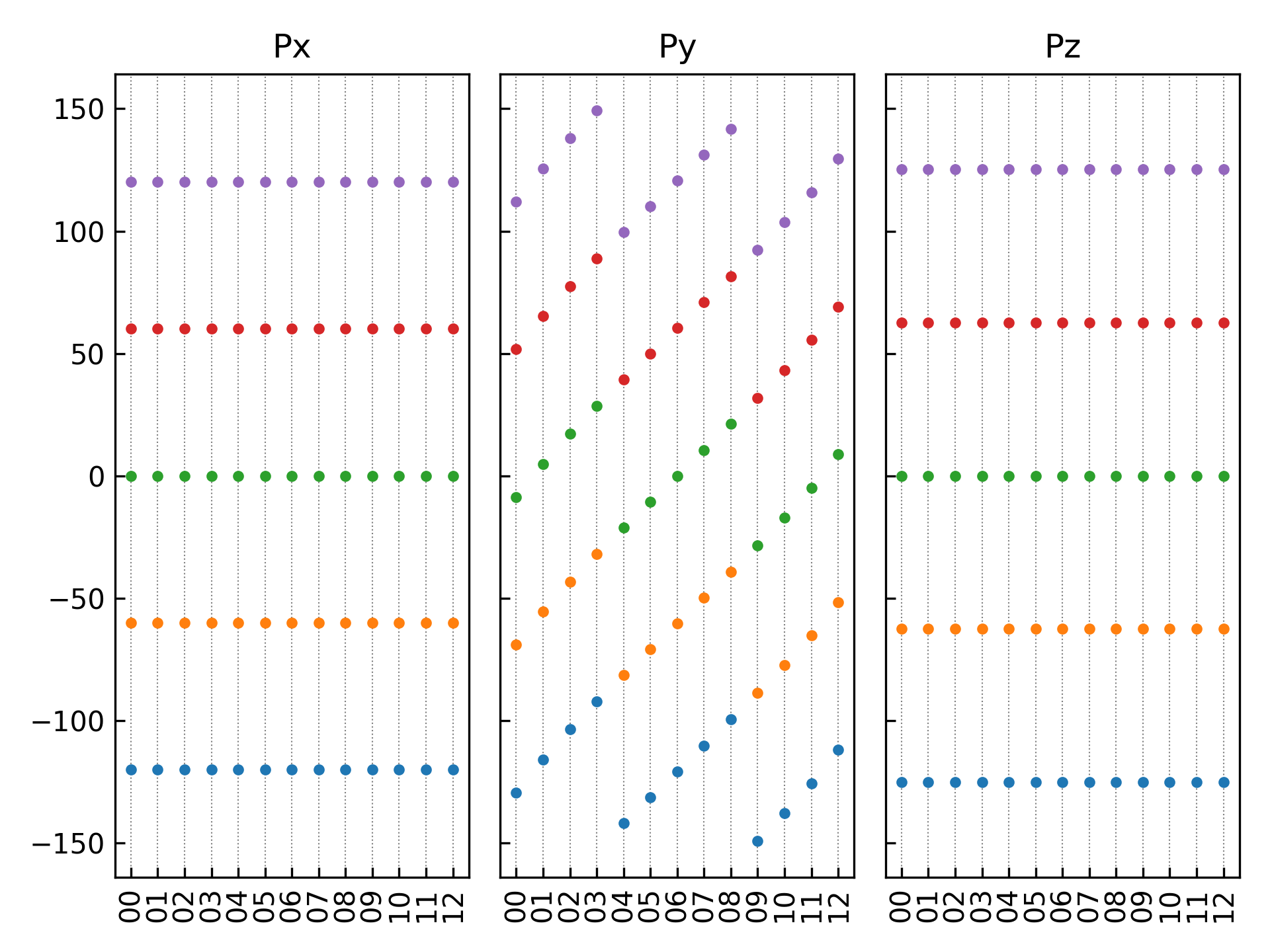
The ferroelectric polarization values for the head and tail configurations can be found below:
1from dspawpy.plot import plot_polarization_figure
2
3python
4plot_polarization_figure(directory='.', annotation=True, annotation_style=1)  # Displays the ferroelectric polarization values for the initial and final configurations.
The code will generate the following combined plot:
Alternatively, a second annotation style can be used:
1from dspawpy.plot import plot_polarization_figure
2
3plot_polarization_figure(directory='.', annotation=True, annotation_style=2)  # Displays the ferroelectric polarization values for the initial and final configurations.
The code will generate the following combined plot:
警告
If you encounter QT-related error messages when executing the above script via SSH connection to a remote server, it may be due to incompatibility between the program used (e.g., MobaXterm) and the QT library. Either change the program (e.g., VSCode or the system’s built-in terminal command line), or add the following code starting from the second line of your Python script:
import matplotlib
matplotlib.use('agg')
8.12 Zero-Point Vibrational Energy Data Processing
Taking the frequency.txt file obtained from a quick start \(CO\) system frequency calculation as an example, the zero-point vibrational energy is calculated based on the following formula:
where \(\nu_i\) are the normal mode frequencies, \(h\) is Planck’s constant (\(6.626\times10^{-34} J\cdot s\)), and \(N\) is the number of atoms.
See
12getZPE.py:1# coding:utf-8 2from dspawpy.io.utils import getZPE 3 4# Import the frequency.txt file obtained from frequency calculation 5getZPE( 6 fretxt="dspawpy_proj/dspawpy_tests/inputs/2.13/frequency.txt", 7)
The code execution results will be saved to the ZPE.dat file, and the file content is as follows:
Data read from D:\quickstart\2.13\frequency.txt
Frequency (meV)
284.840038

--> Zero-point energy,  ZPE (eV): 0.142420019
8.13 TS Hot Calibration Energy
Contribution of the entropy change of the adsorbate to the energy
Calculation is based on the following formula:
Here, \(\Delta S_{a d s}\) represents the entropy change of the adsorbate, calculated based on the harmonic approximation. \(S_{v i b}\) represents the vibrational entropy. \(\nu_i\) is the normal mode frequency, \(N_A\) is Avogadro’s constant (\(6.022\times10^{23} mol^{-1}\)), \(h\) is Planck’s constant (\(6.626\times10^{-34} J\cdot s\)), \(k_B\) is the Boltzmann constant (\(1.38\times10^{-23} J\cdot K^{-1}\)), \(R\) is the ideal gas constant (\(8.314 J\cdot mol^{-1}\cdot K^{-1}\)), and \(T\) is the system temperature in units of \(K\).
See
13getTSads.pyfor reference:1# coding:utf-8 2from dspawpy.io.utils import getTSads 3 4# Import the frequency.txt file calculated from frequency, temperature can be modified arbitrarily 5getTSads( 6 fretxt="dspawpy_proj/dspawpy_tests/inputs/2.13/frequency.txt", 7 T=298.15, 8)
The execution result will be saved to the TS.dat file, with the following content:
Data read from D:\quickstart\2.13\frequency.txt
Frequency (THz)
68.873994

--> Entropy contribution,  T*S (eV): 4.7566990201851275e-06
Ideal gas entropy contribution to energy
Calculations are based on the following formula:
Where:
where \(I_A\) to \(I_C\) are the three principal moments of inertia for a non-linear molecule, \(I\) is the degenerate moment of inertia for a linear molecule, and \(\sigma\) is the symmetry number of the molecule. Furthermore, monatomic refers to a monatomic molecule, linear refers to a linear molecule, and nonlinear refers to a non-linear molecule. total spin is the total spin quantum number. vib DOF represents vibrational degrees of freedom.
Refer to the
13getTSgas.pyscript for processing:1# coding:utf-8 2from dspawpy.io.utils import getTSgas 3 4# Read elements and coordinates from the calculation result file (json or h5) 5TSgas = getTSgas( 6 fretxt="dspawpy_proj/dspawpy_tests/inputs/2.13/frequency.txt", 7 datafile="dspawpy_proj/dspawpy_tests/inputs/2.13/frequency.h5", 8 potentialenergy=-0.0, 9 geometry="linear", 10 symmetrynumber=1, 11 spin=1, 12 temperature=298.15, 13 pressure=101325.0, 14) 15print("Entropy contribution, T*S (eV):", TSgas) 16 17# If only the frequency.txt file is available, the calculation can be completed by manually specifying the elements and coordinates 18# TSgas = getTSgas(fretxt='dspawpy_proj/dspawpy_tests/inputs/2.13/frequency.txt', datafile=None, potentialenergy=-0.0, elements=['H', 'H'], geometry='linear', positions=[[0.0, 0.0, 0.0], [0.0, 0.0, 1.0]], symmetrynumber=1, spin=1, temperature=298.15, pressure=101325.0)
8.14 Appendix
Quickly download all scripts by clicking
UserScripts.zip