3 Application Cases

This chapter presents various application examples of DS-PAW, including how to calculate magnetic moments and how to calculate antiferromagnetic materials. Users can gain a deeper understanding of DS-PAW software through the following application tutorials.

3.1 Calculation of the Magnetic Moment of Atom \(O\)

This section introduces the calculation of magnetic systems using a single oxygen atom as an example.

File Preparation for Self-Consistent Calculation of an \(O\) Atom

Since this calculation involves the magnetic moment of a single oxygen atom, structural relaxation is not necessary. We proceed directly to the self-consistent field (SCF) calculation. Prepare the input files scf.in and structure.as. scf.in is as follows:

task = scf
sys.symmetry = false
sys.structure = structure.as
sys.spin = collinear
cal.smearing = 1
cal.sigma = 0.01
cal.kpoints = [1, 1, 1]

The following parameters in the input file are crucial for this calculation:

• sys.symmetry: DS-PAW can reduce computational cost by using symmetry, but it may also lead to unreasonable results such as energy degeneracy. Symmetry is turned off in this calculation;

• sys.spin: Specifies the system's magnetism as collinear.

• cal.kpoints: For non-periodic dimensions, the k-point can be set to 1;

The structure.as file is referenced as follows:

Total number of atoms
1
Lattice
7.50000000 0.00000000 0.00000000
0.00000000 8.00000000 0.00000000
0.00000000 0.00000000 8.90000000
Cartesian
O  0.00000000 0.00000000 0.00000000

The structure file uses Cartesian coordinates, hence the coordinate type in line 7 is Cartesian; to minimize symmetry in the structure, the lattice was modified to a [7.5, 8, 8.9] lattice.

Run the program

After preparing the input files, upload the scf.in and structure.as files to the environment where DS-PAW is installed, and run the DS-PAW scf.in command.

Analysis of calculation results.

After the calculation based on the input files is completed, output files such as DS-PAW.log and scf.h5 will be generated.

Open the scf.h5 file with HDFView, and the Eigenvalue data will be as follows:

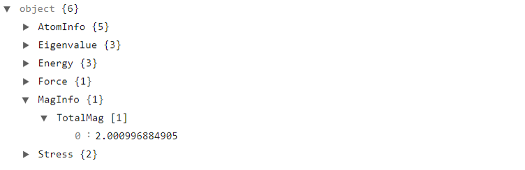
The number of up-spin electrons is 4 and the number of down-spin electrons is 2, obtained from the Eigenvalue - Spin - Occupation section of scf.h5. The total magnetic moment is \(2\mu B\), obtained from the MagInfo section of scf.h5, and also confirmed as \(2 \mu B\) in DS-PAW.log.

3.2 \(NiO\) antiferromagnetic calculation

This section will introduce how to set up antiferromagnetic calculations using the NiO system as an example.

Self-consistent calculation for the \(NiO\) system

This case omits the structure relaxation process; users should perform a structure relaxation calculation first when reproducing this case. Prepare the parameter file scf.in and the structure file structure.as, and the scf.in file is as follows:

task = scf
sys.structure = structure.as
sys.spin = collinear
cal.smearing = 4
cal.kpoints = [8, 8, 8]
cal.cutoff = 650

The following parameters in the input file of this calculation require special attention:

• cal.smearing: The tetrahedron method with Bloechl correction is employed in this calculation, and sigma will be forced to 0 when using this method.

• sys.spin: Specifies the magnetism of the system. NiO is an antiferromagnetic material, so the magnetism is set to collinear;

• cal.cutoff: Sets the plane-wave cutoff to 650 eV.

Refer to the structure.as file as follows:

Total number of atoms
4
Lattice
4.16840000 2.08420000 2.08420000
2.08420000 4.16840000 2.08420000
2.08420000 2.08420000 4.16840000
Cartesian Mag
Ni 1.04210000 1.04210000 1.04210000   2.0
Ni 5.21050000 5.21050000 5.21050000   -2.0
O 3.12630000 3.12630000 3.12630000    0
O 7.29470000 7.29470000 7.29470000    0

To set the magnetic moments, add the Mag tag after Cartesian on the seventh line of the structure file. Then, set the magnetic moment for each atom on the line containing its coordinates. Because we need to represent antiferromagnetism (the entire system does not show a net magnetic moment, but individual atoms have magnetic moments), this example uses a unit cell of 4 atoms. The magnetic moments for the 4 Ni atoms are set to 2, -2, 0, 0.

备注

1. The Mag tag allows setting the magnetic moments for each atom in the system. For collinear spin calculations, the total magnetic moment of each atom can be added. For spin-orbit coupling calculations, the magnetic moments in the x, y, and z directions need to be added using the tags Mag_x, Mag_y, and Mag_z. Add the magnetic moments in the three directions after the corresponding atomic coordinates. Taking the NiO system as an example, if a spin-orbit coupling calculation is performed, the magnetic moment settings should be as follows:

Total number of atoms
4
Lattice
4.16840000 2.08420000 2.08420000
2.08420000 4.16840000 2.08420000
2.08420000 2.08420000 4.16840000
Cartesian Mag_x Mag_y Mag_z
Ni 1.04210000 1.04210000 1.04210000   0.0 0.0 2.0
Ni 5.21050000 5.21050000 5.21050000   0.0 0.0 -2.0
O 3.12630000 3.12630000 3.12630000    0.0 0.0 0.0
O 7.29470000 7.29470000 7.29470000    0.0 0.0 0.0

run the program

After preparing the input files, upload the :guilabel:`scf.in` and :guilabel:`structure.as` files to the environment where DS-PAW is installed, and run the command :guilabel:`DS-PAW scf.in`.

Analysis of self-consistent field (SCF) calculation results

Based on the input file described above, after the calculation is completed, the following output files will be generated: DS-PAW.log and scf.h5, etc. From DS-PAW.log, the total magnetic moment after the self-consistent calculation can be read as \(1e-8 \mu B\), which is almost 0.

\(NiO\) Density of States Calculation

After that, we will prepare for the density of states (DOS) calculation, preparing the parameter file pdos.in, the structure file structure.as, and the charge density file rho.bin obtained from the self-consistent calculation. The pdos.in file is as follows:

task = dos
sys.structure = structure.as
sys.spin = collinear
cal.iniCharge = ./rho.bin
cal.smearing = 4
cal.kpoints = [16, 16, 16]
cal.cutoff = 650
dos.range = [-20, 20]
dos.resolution = 0.05
dos.project = true

pdos.in Input Parameters:

• dos.range: Specifies the energy range for DOS calculation, from -20 to 20 eV.

• dos.resolution : indicates the interval precision for sampling within the energy calculation range;

• dos.project: Controls the projection calculation for the density of states; projection for the density of states is enabled in this calculation.

run the program

Upload the newly created pdos.in file to the server, and then run the command DS-PAW pdos.in.

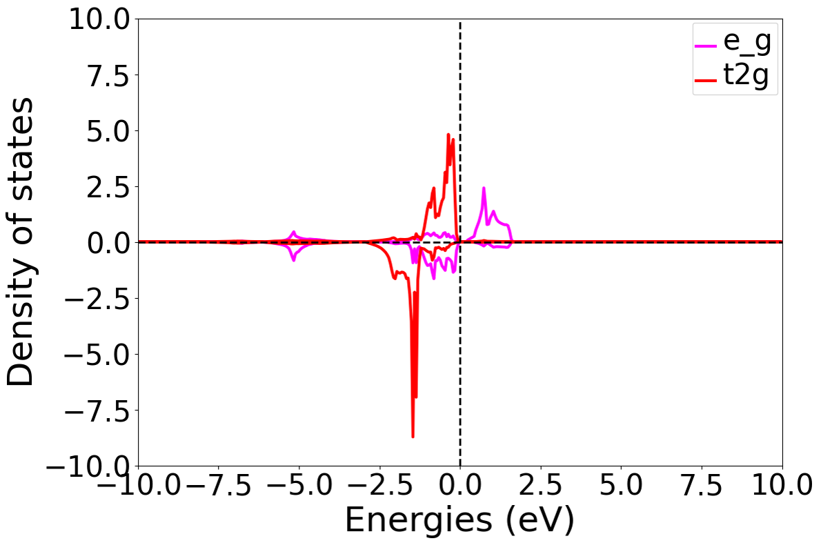
Analysis of DOS (Density of States) Calculation Results

After completing the calculation based on the input file, output files such as DS-PAW.log and dos.h5 will be generated. Using the relevant scripts in Auxiliary Tool User Guide to process the dos.h5 file and analyze the t2g and eg orbitals of the 2nd Ni atom, the density of states distribution shown below is obtained. This is the result without a U value applied:

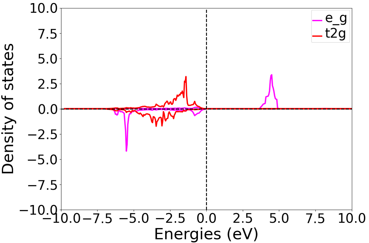
\(NiO\) system DFT+U density of states calculation

The calculation procedure for the density of states (DOS) of the NiO system using DFT+U is the same as that described in the previous section for the NiO system, with the difference being that DFT+U parameters need to be included in both the self-consistent field (SCF) calculation and the DOS calculation. The input parameters that need to be added are as follows:

#correction related
corr.dftu=true
corr.dftuForm = 1
corr.dftuElements =[Ni]
corr.dftuOrbital=[d]
corr.dftuU = [8]
corr.dftuJ = [0.95]

Here are a few parameters in the input file that require special attention for this calculation:

• corr.dftu sets the switch for turning on DFT+U, which is set to true in this example;

• corr.dftuForm sets the DFT+U method, with 1 corresponding to the DFT+U+J method (Liechtenstein’s formulation);

• corr.dftuElements sets the elements to which U is applied, which is Ni in this example;

• corr.dftuOrbital specifies the orbitals to which the U correction is applied, which is set to d orbitals in this example;

• corr.dftuU sets the specific U value, which is set to 8 in this example;

• corr.dftuJ sets the specific J value, which is set to 0.95 in this example;

After the self-consistent field (SCF) and density of states (DOS) calculations are completed, the distribution of the t2g and eg orbital density of states for the second Ni atom after the DFT+U calculation is analyzed. The resulting distribution plot is shown below:

备注

1. DFT+U allows setting U values for multiple elements and their corresponding orbitals. For example, to set U=8 and J=0.95 for Ni's d orbitals, and U=1 and J=0 for O's p orbitals, the settings are as follows: corr.dftuElements = [Ni,O] corr.dftuOrbital = [d,p] corr.dftuU = [8,1] corr.dftuJ = [0.95,0].

2. The default DFT+U method is DFT+U (Dudarev’s formulation), corresponding to the parameter corr.dftuForm = 2. When using this method, the J value is forced to be 0, so setting the J value is invalid in this case.

3.3 \(AuAl\) slab model work function calculation

This section will demonstrate how to calculate the work function using the \(AuAl\) slab model as an example.

File Preparation for Self-Consistent Calculation of the \(AuAl\) Slab Model

This case omits the structure relaxation process; users need to perform structure relaxation calculations before reproducing this case. Prepare the parameter file scf.in and the structure file structure.as. The scf.in file is as follows:

task = scf
sys.structure = structure.as
sys.spin = collinear
cal.smearing = 4
cal.kpoints = [8, 8, 1]
cal.cutoff = 530

io.potential=true
potential.type = hartree

#correction related
corr.dipol = true
corr.dipolDirection = c

The following parameters in the input file of this calculation require special attention:

• io.potential is the switch for calculating the potential function in the self-consistent field (SCF) calculation;

• potential.type controls the type of potential function to be saved. The electrostatic potential data is needed when calculating the work function, and here we set potential.type = hartree;

• corr.dipol is the switch for dipole correction; set to true in this example;

• corr.dipolDirection In this example, the direction of the dipole correction is set to the c direction of the lattice vectors.

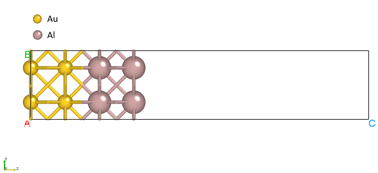
The structure.as file is referenced as follows:

Total number of atoms
8
Lattice
 4.06384898 0.00000000 0.00000000
 0.00000000 4.06384898 0.00000000
 0.00000000 0.00000000 20.00000000
Cartesian
Au 1.01596223 1.01596223 0.00000000
Au 3.04788672 3.04788672 0.00000000
Au 3.04788672 1.01596224 2.03914999
Au 1.01596224 3.04788672 2.03914999
Al 1.01596224 1.01596224 4.07109999
Al 3.04788673 3.04788673 4.07109999
Al 3.04788673 1.01596224 6.09585000
Al 1.01596224 3.04788673 6.09585000

The structure is shown in the figure below:

run program execution

After preparing the input files, upload the scf.in and structure.as files to the environment where DS-PAW is installed and run the command DS-PAW scf.in.

workfunction data analysis

After the calculation based on the above input files, the output files such as DS-PAW.log and scf.h5 will be generated. Processing the data from scf.h5 yields the work function.

You can use a python script to analyze the scf.h5 file, averaging the 3D potential function in-plane. See the Auxiliary Tool User Guide section for specific instructions. The resulting vacuum direction potential curve is shown below:

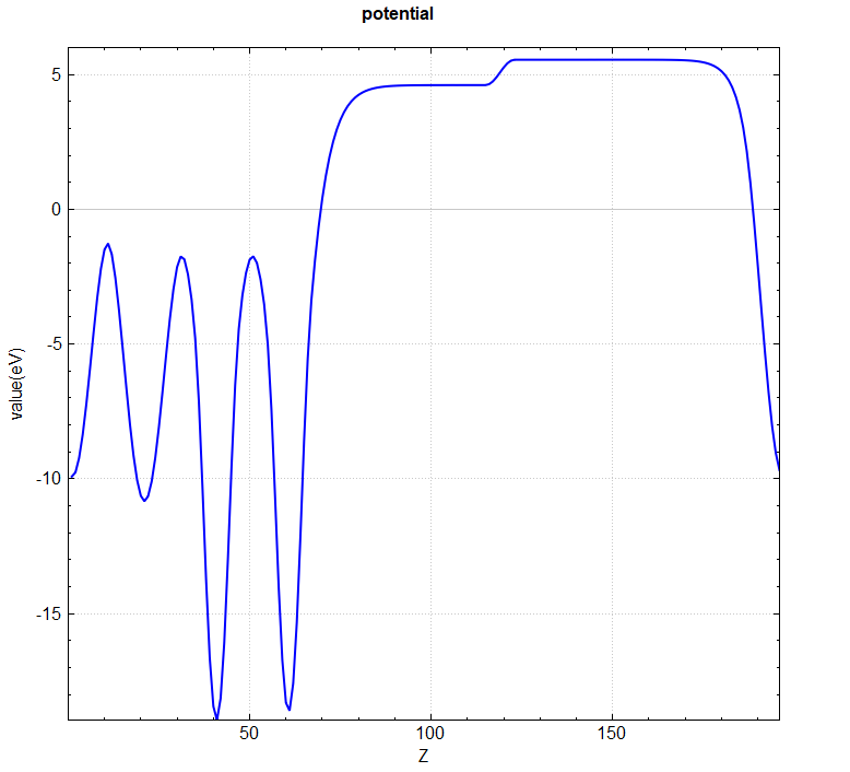
From the in-plane averaged potential plot, the vacuum potentials for Au and Al are 5.5 eV and 4.6 eV, respectively.

The Fermi level can be read from scf.h5 as 0.113 eV.

Based on the formula \(w=-e \phi-E_F\), the work function of Au in the \(AuAl\) slab model is 5.387 eV, and that of Al is 4.487 eV. The literature values [1] are: Au's work function in the range of 5.10-5.47 eV, and Al's work function in the range of 4.06-4.26 eV.

3.4 \(Ru-N4\) Computational Electrocatalysis of Nitrogen Reduction Reaction

This section will demonstrate how to simulate an electrocatalytic nitrogen reduction reaction (eNRR) using DS-PAW. The reaction uses a carbon-based supported transition metal Ru single atom as a catalyst, and DS-PAW is used to simulate the adsorption and reduction process of nitrogen molecules.

During electrochemical interfacial reactions, the interface is typically connected to an external electrode with a constant electrode potential. To ensure that the electronic chemical potential equilibrates with the external electrode potential, meaning the grand canonical ensemble for electrons, there will be an influx and outflux of electrons in the actual system. Traditional first-principles calculations are usually performed under the canonical ensemble, i.e., under the condition of charge conservation, and thus cannot accurately describe electrochemical interfacial reactions. We will refer to the calculation model expanded under charge conservation as the constant charge model (CCM).

Since the constant charge model is not suitable for handling electrochemical interface problems, we can adopt first-principles calculations expanded in the electronic grand canonical ensemble. This calculation method is also known as the fixed potential method/constant potential method. In this case, we will refer to the fixed potential calculation model as the constant potential model (CPM).

Flow Calculation Procedure and Input Files

This example simulates the adsorption and reduction of nitrogen molecules on a carbon-supported transition metal Ru single atom catalyst using DS-PAW. The simulated reaction is the adsorption of nitrogen molecules on a carbon-supported Ru single atom, which can be simplified as: \((Ru-N_4) + N_2 = (Ru-N_4-N_2)\). Three different models, CCM_vacuum, CCM_water, and CPM_water, are used in the calculation. The entire calculation procedure can be roughly divided into four steps, detailed as follows:

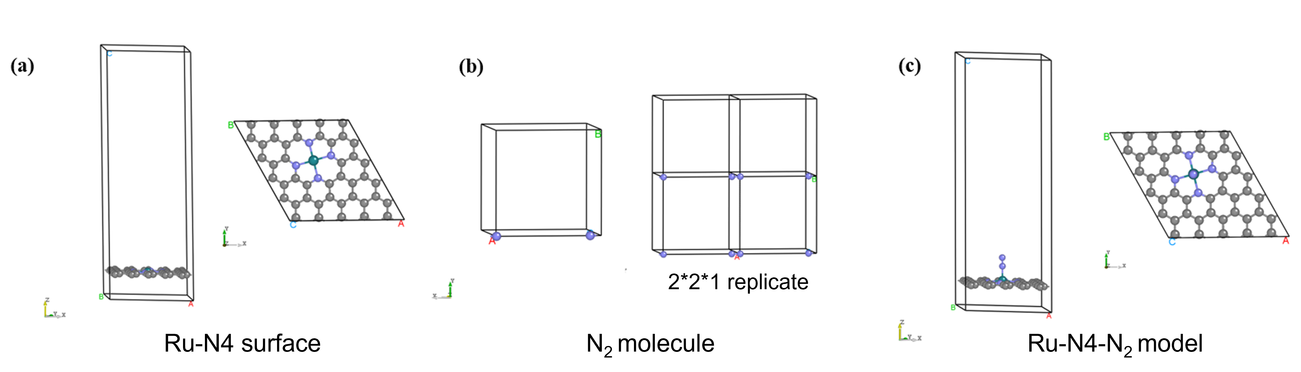
Build the model

The models include: (a) a carbon-supported Ru atom model (\(Ru-N_4\)), (b) a single \(N_2\) molecule model, and (c) a carbon-supported Ru atom model with adsorbed \(N_2\) molecule (\(Ru-N_4-N_2\)). The model structures are shown below:

Relaxation Structure Relaxation

Perform structural relaxation on the constructed structure to obtain a stable structure. Core parameters required for structural relaxation in DS-PAW:

relax.max =  200                  # Specify the maximum number of ionic steps for structure relaxation
relax.freedom = atom              #Specify the degree of freedom for structural relaxation
relax.convergence =  0.02         #Specifies the convergence criterion for atomic forces during structural relaxation
relax.methods = CG                # Conjugate gradient method is specified for structural relaxation.

Energy Calculation

Energy calculations were performed under different model conditions to obtain the energies of stable configurations. The results are presented below, categorized by model.

CCM_vacuum

Standard scf calculation under vacuum layer to obtain the energy under the CCM_vacuum model. The core parameters required for a single point energy calculation in DS-PAW are listed below:

task = scf

# Self-consistent field calculation related
cal.methods = 1                   #Specifies the self-consistent electronic part optimization method as BD (block Davidson) method
cal.smearing = 1                  # Specifies Gaussian smearing to set the fractional occupation of each wavefunction
cal.k_sampling = G                  #Specifies the method for generating the Brillouin zone k-point grid
cal.kpoints = [2, 2, 1]           #Specifies the size of the k-point grid sampling in the Brillouin zone

cal.cutoffFactor = 1.0            # Specifies the coefficient for the plane-wave basis cutoff energy parameter cal.cutoff


corr.VDW = true                   # Specifies that van der Waals correction calculation is enabled.
corr.VDWType = D2G                #Specifies the Grimme's DFT-D2 method for van der Waals correction

CCM_water

In the CCM model, implicit solvation models can also be used to consider solvent effects. Here, we take an aqueous solution as an example and list the core parameters that need to be set to introduce the solvation model in the SCF calculation using DS-PAW:

task = scf

# Solvation model related
sys.sol = true                         # Specify whether to apply the implicit solvation model, true means enabled.
sys.solEpsilon = 78.4                  # Specify the dielectric constant of the solvent, 78.4 for water
sys.solLambdaD = 3.04                  # Specify the Debye length in the Poisson-Boltzmann equation, in Å
sys.solTAU = 0                         # Specify the magnitude of the effective interfacial tension per unit area, in eV/Å^2
io.boundCharge = false                 # Specify whether to output the solvent-bound charge density file, false means off.

CPM_water

In DS-PAW, the energy under the CPM model can be obtained by using the fixed potential method. In the newly released 2023A version, the fixed potential calculation must introduce a solvation model. Here are the core parameters for fixed potential calculations in an implicit aqueous environment using DS-PAW:

task = scf
# Solvent model related
sys.sol = true                         # Specify whether to apply the implicit solvation model, true means enabled.
sys.solEpsilon = 78.4                  # Specifies the dielectric constant of the solvent, with a default value of 78.4 for water.
sys.solLambdaD = 3.04                  #Specifies the Debye length in the Poisson-Boltzmann equation, in Å
sys.solTAU = 0                         # Specifies the effective interfacial tension per unit area, in eV/Å^2
io.boundCharge = false                 # Specifies whether to output the solvent bound charge density file, false means off

# Related to fixed potential settings
sys.fixedP = true                      # Specifies whether to enable fixed potential calculation, true means enabled
sys.fixedPConvergence = 0.01           # Specifies the convergence criterion for the fixed potential calculation. The calculation ends when the delta_electron between two self-consistent calculations is less than the convergence criterion.
sys.fixedPMaxIter = 60                 #Specify the maximum number of iterations for fixed potential calculation.
sys.fixedPPotential = 0                # Specifies the target electrode potential value for the fixed potential calculation, using SHE as the reference electrode potential by default.
sys.fixedPType = SHE                   # Specifies the potential type for the potential value given by sys.fixedPPotential, supporting SHE (Standard Hydrogen Electrode) and PZC (Potential of Zero Charge)

ReactionEnergy Calculation

This example selects three different computational models. First, the adsorption reaction equations for each model are introduced:

CCM_vacuum

In this model, the adsorption reaction can be written as:

\((Ru-N4) + N2 (ideal gas) = (Ru-N4-N2)\)

We define \({\Delta}E\) as the reaction energy, and the calculation expression for the reaction energy is:

\({\Delta}E = E0(Ru-N4-N2) - E0(Ru-N4) - E0(N2)\)

where E0 corresponds to the total energy of the system in the vacuum model ( \(\sigma\) →0), which can be obtained from the self-consistent calculation results in the scf.h5 or system.json file by searching for the keyword "TotalEnergy0".

CCM_water

Under this model, the adsorption reaction equation can be written as:

\((Ru-N4)(in water) + N2 (ideal gas) = (Ru-N4-N2) (in water)\)

\({\Delta}E = E0(Ru-N4-N2) - E0(Ru-N4) - E0(N2)\)

Where, E0 corresponds to the total energy of the system under the model of aqueous solution immersion ( \(\sigma\) →0), this value can be obtained from the self-consistent field calculation, specifically from the scf.h5 or system.json file, by searching for the keyword "TotalEnergy0".

CPM_water

The reaction process simulated in this model is the adsorption of \(N_2\) in the gas phase on a catalyst surface wetted by an aqueous solution and in contact with a 0V vs. SHE (Standard Hydrogen Electrode) electrode. Two different adsorption reaction equations can be written for this process. For ease of description, we define the following physical quantity symbols:

• \(ne0\) : Number of core electrons in the neutral system.

• \(ne\) : Total number of electrons in the system when the system voltage is set (value set by sys.fixedPPotential, corresponding to 0 V in this example)

• \(dne\) : The charge of the system at the set system voltage: \(dne = ne - ne0\)

• \(\mu_e\) : Electronic chemical potential of the system, with the potential zero point at the bulk solution (i.e., the potential value at the lowest charge density point obtained from DFT calculations)

• \({\Delta}e\) : Difference in the number of valence electrons between the adsorbed system (eAB) and the sum of valence electrons of the substrate and adsorbate (eA+eB).

• \(\Omega0\) : grand total energy(sigma→0): the total energy of the system in the grand canonical ensemble of electrons, which is expressed as: \(\Omega0 = E0-dne*\mu_e\)

In this case, the adsorption reaction formula under the CPM_water model can be written as follows:

Method 1, considering \({\Delta}e\) in the reaction equation, the adsorption reaction can be written as:

\(Ru-N4 (0V vs. SHE) + N2(ideal gas) = Ru-N4-N2 (0V vs. SHE) - {\Delta}e\)

\({\Delta}E = E0(Ru-N4-N2) - {\Delta}e*\mu_e - E0(Ru-N4) - E0(N2)\)

The values of E0 can be obtained from the self-consistent calculation results in the scf.h5 or system.json file, by searching for the keyword "TotalEnergy0".

The values of \(ne\) and \(\mu_e\) can be obtained from the self-consistent calculation results in the DS-PAW.log file (or scf.h5 or system.json), by searching for the keywords "Electron" and "Chemical Potential(electron)" under the last LOOP.

Method two, considering the total energy of the system \(\Omega0\) in the grand canonical ensemble of electrons.

Since the constant potential calculation simulates the electronic grand canonical ensemble, the total energy \(E0\) in the reaction energy calculation should be replaced by \(\Omega0\). The adsorption reaction equation can be written as:

\((Ru-N4) (0V vs. SHE) + N2(ideal gas) = (Ru-N4-N2) (0V vs. SHE)\)

\({\Delta}E = \Omega0(Ru-N4-N2) - \Omega0(Ru-N4) - \Omega0(N2)\)

Where the value of \(\Omega0\) can be obtained from the self-consistent calculation in the DS-PAW.log file (or the scf.h5 or system.json files), by searching for the keyword "Grand Total Energy" in the last LOOP.

Since the potential of (Ru-N4) versus (Ru-N4-N2) is 0V vs. SHE, a fixed potential calculation at 0V is performed for (Ru-N4) and (Ru-N4-N2). Data is extracted from the corresponding output files of DS-PAW, and the following table is obtained, with energy units in eV:

system	\(E0\)	\(nE0\)	\(ne\)	\(dne\)	\(\mu_e\)	\(\Omega0\)
N2	-545.9393	10	/	/	/	-545.9393
Ru-N4	-10572.2452	212	211.224	-0.776	-4.60223	-10575.81654
Ru-N4-N2	-11119.6117	222	221.229	-0.771	-4.60054	-11123.15868

Next, we substitute the data from Table 1 into the corresponding expressions for calculation:

Method 1 Considering \({\Delta}e\) in the reaction equation, the reaction energy calculation process is as follows:

\(Ru-N4 (0V vs. SHE) + N2(ideal gas) = Ru-N4-N2 (0V vs. SHE) - {\Delta}e\)

\({\Delta}E = E0(Ru-N4-N2) - {\Delta}e*\mu_e - E0(Ru-N4) - E0(N2)\)

\(= -11119.6117-(221.229-211.224-10)*(-4.600)-(-10572.2452)-(-545.9393)\)

\(= - 1.4042 eV\)

Method 2 Consider the grand canonical potential \(\Omega0\) of the system, and the reaction energy calculation is as follows:

\((Ru-N4) (0V vs. SHE) + N2(ideal gas) = (Ru-N4-N2) (0V vs. SHE)\)

\({\Delta}E = \Omega0(Ru-N4-N2) - \Omega0(Ru-N4) - \Omega0(N2)\)

\(= -11123.1586-(-10575.8165)-(-545.9393)\)

\(= -1.4027 eV\)

The calculated adsorption energies obtained using the two methods are consistent. It is apparent that the reaction energy under a fixed potential can be easily computed using \(\Omega0\) as defined in DS-PAW.

Run the program

After preparing the input files, upload the in files for structural relaxation calculations, energy calculations, and fixed potential calculations, along with the structure.as structure file, to an environment with DS-PAW installed. Following the workflow, run the DS-PAW input.in command in multiple steps or submit job scripts to complete multiple calculations.

ReactionEnergy Reaction Energy data analysis

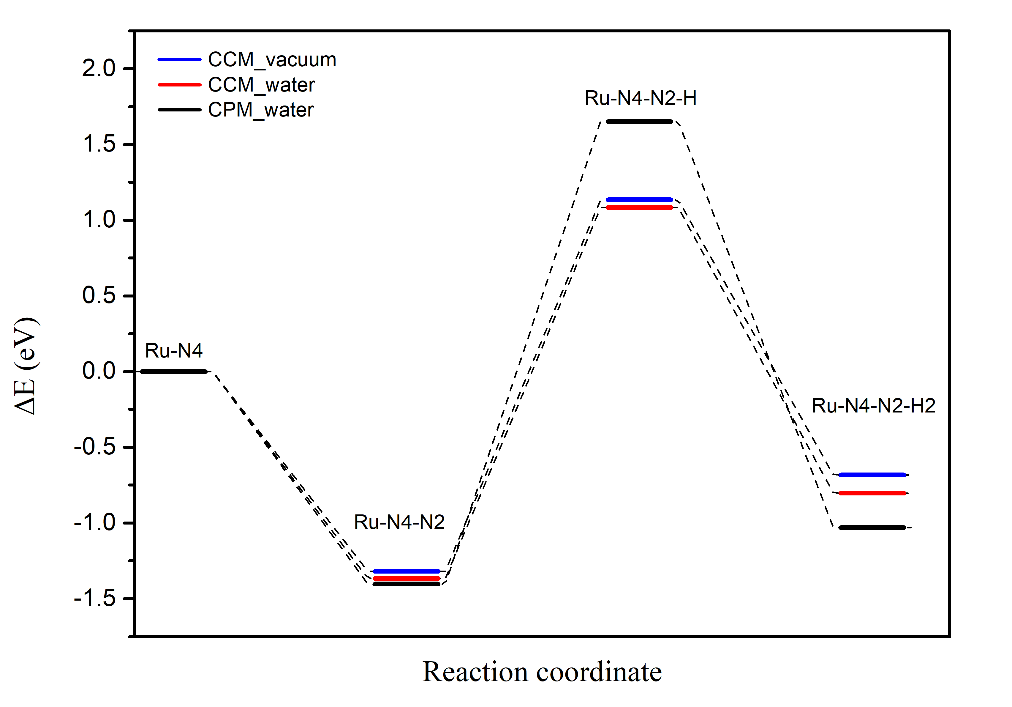
Substituting the data from Table 1 into the adsorption reaction equations for the CCM_vacuum, CCM_water, and CPM_water models, we calculate the reaction energies of the first three steps of the eNRR for the three models. The results are shown in Table 2:

reaction/ \({\Delta}e\) (eV)	CCM_vacuum	CCM_water	CPM_water
\((Ru-N4) + N2 = (Ru-N4-N2)\)	-1.3180	-1.3668	-1.4027
\((Ru-N4-N2) + 0.5H2 = (Ru-N4-N2-H)\)	1.1355	1.0833	1.6511
\((Ru-N4-N2-H) +0.5H2 = (Ru-N4-N2-H2)\)	-0.6833	-0.8030	-1.0305

The results are then plotted as a reaction coordinate curve, as shown in Figure 3:

3.5 ref References

[1]

William M Haynes, David R Lide, and Thomas J Bruno. CRC handbook of chemistry and physics. CRC press, 2016. doi:10.1201/9781315380476.